Tuning Java DB
Version 10.5
Derby Document build:
July 29, 2009, 11:16:10 AM (EDT)


Version 10.5   Tuning Java DB
   
Contents
Copyright    
License    
Relationship between Java DB and Derby    
About this guide    
Purpose of this guide    
Audience    
How this guide is organized    
Performance tips and tricks    
The tips    
Use prepared statements with substitution parameters    
Create indexes, and make sure they are being used    
Increase the size of the data page cache    
Tune the size of database pages    
Avoid expensive queries    
Use the appropriate getXXX and setXXX methods for the type    
Tune database booting/class loading    
Avoid inserts in autocommit mode if possible    
Customize the optimizer methods for table functions    
More tips    
Shut down the system properly    
Put Derby first in your classpath    
Tuning databases and applications    
Application and database design issues    
Avoiding table scans of large tables    
Avoiding compiling SQL statements    
Shielding users from Derby class-loading events    
Analyzing statement execution    
Working with RunTimeStatistics    
Overview    
How you use the RUNTIMESTATISTICS attribute    
Analyzing the information    
DML statements and performance    
Performance and optimization    
Index use and access paths    
Joins and performance    
Derby's cost-based optimization    
Locking and performance    
Transaction-based lock escalation    
Locking a table for the duration of a transaction    
Non-cost-based optimizations    
Non-cost-based sort avoidance (tuple filtering)    
The MIN() and MAX() optimizations    
Overriding the default optimizer behavior    
Selectivity and cardinality statistics    
Determinations of rows scanned from disk for a table scan    
How the optimizer determines the number of rows in a table    
Estimations of rows scanned from disk for an index scan    
Queries with a known search condition    
Queries with an unknown search condition    
Statistics-based versus hard-wired selectivity    
Selectivity from cardinality statistics    
Selectivity from hard-wired assumptions    
What are cardinality statistics?    
Working with cardinality statistics    
When cardinality statistics are automatically updated    
When cardinality statistics go stale    
Internal language transformations    
Predicate transformations    
BETWEEN transformations    
LIKE transformations    
Simple IN predicate transformations    
NOT IN predicate transformations    
OR transformations    
Transitive closure    
Transitive closure on join clauses    
Transitive Closure on Search Clauses    
View transformations    
View flattening    
Predicates pushed into views or derived tables    
Subquery processing and transformations    
Materialization    
Flattening a subquery into a normal join    
Flattening a subquery into an EXISTS join    
Flattening VALUES subqueries    
DISTINCT elimination in IN, ANY, and EXISTS subqueries    
IN/ANY subquery transformation    
Outer join transformations    
Sort avoidance    
DISTINCT elimination based on a uniqueness condition    
Combining ORDER BY and DISTINCT    
Combining ORDER BY and UNION    
Aggregate processing    
COUNT(nonNullableColumn)    
Trademarks    


Tuning Java DB
Apache Software FoundationTuning Java DBApache Derby
Copyright
Copyright 2004-2009 The Apache Software Foundation
Copyright 2009 Sun Microsystems, Inc., 4150 Network Circle, Santa Clara, California 95054, U.S.A.
Licensed under the Apache License, Version 2.0 (the "License"); you may not use this file except in compliance with the License. You may obtain a copy of the License at http://www.apache.org/licenses/LICENSE-2.0.
Related information
License
The Apache License, Version 2.0
Apache License Version 2.0, January 2004 http://www.apache.org/licenses/ TERMS AND CONDITIONS FOR USE, REPRODUCTION, AND DISTRIBUTION 1. Definitions. "License" shall mean the terms and conditions for use, reproduction, and distribution as defined by Sections 1 through 9 of this document. "Licensor" shall mean the copyright owner or entity authorized by the copyright owner that is granting the License. "Legal Entity" shall mean the union of the acting entity and all other entities that control, are controlled by, or are under common control with that entity. For the purposes of this definition, "control" means (i) the power, direct or indirect, to cause the direction or management of such entity, whether by contract or otherwise, or (ii) ownership of fifty percent (50%) or more of the outstanding shares, or (iii) beneficial ownership of such entity. "You" (or "Your") shall mean an individual or Legal Entity exercising permissions granted by this License. "Source" form shall mean the preferred form for making modifications, including but not limited to software source code, documentation source, and configuration files. "Object" form shall mean any form resulting from mechanical transformation or translation of a Source form, including but not limited to compiled object code, generated documentation, and conversions to other media types. "Work" shall mean the work of authorship, whether in Source or Object form, made available under the License, as indicated by a copyright notice that is included in or attached to the work (an example is provided in the Appendix below). "Derivative Works" shall mean any work, whether in Source or Object form, that is based on (or derived from) the Work and for which the editorial revisions, annotations, elaborations, or other modifications represent, as a whole, an original work of authorship. For the purposes of this License, Derivative Works shall not include works that remain separable from, or merely link (or bind by name) to the interfaces of, the Work and Derivative Works thereof. "Contribution" shall mean any work of authorship, including the original version of the Work and any modifications or additions to that Work or Derivative Works thereof, that is intentionally submitted to Licensor for inclusion in the Work by the copyright owner or by an individual or Legal Entity authorized to submit on behalf of the copyright owner. For the purposes of this definition, "submitted" means any form of electronic, verbal, or written communication sent to the Licensor or its representatives, including but not limited to communication on electronic mailing lists, source code control systems, and issue tracking systems that are managed by, or on behalf of, the Licensor for the purpose of discussing and improving the Work, but excluding communication that is conspicuously marked or otherwise designated in writing by the copyright owner as "Not a Contribution." "Contributor" shall mean Licensor and any individual or Legal Entity on behalf of whom a Contribution has been received by Licensor and subsequently incorporated within the Work. 2. Grant of Copyright License. Subject to the terms and conditions of this License, each Contributor hereby grants to You a perpetual, worldwide, non-exclusive, no-charge, royalty-free, irrevocable copyright license to reproduce, prepare Derivative Works of, publicly display, publicly perform, sublicense, and distribute the Work and such Derivative Works in Source or Object form. 3. Grant of Patent License. Subject to the terms and conditions of this License, each Contributor hereby grants to You a perpetual, worldwide, non-exclusive, no-charge, royalty-free, irrevocable (except as stated in this section) patent license to make, have made, use, offer to sell, sell, import, and otherwise transfer the Work, where such license applies only to those patent claims licensable by such Contributor that are necessarily infringed by their Contribution(s) alone or by combination of their Contribution(s) with the Work to which such Contribution(s) was submitted. If You institute patent litigation against any entity (including a cross-claim or counterclaim in a lawsuit) alleging that the Work or a Contribution incorporated within the Work constitutes direct or contributory patent infringement, then any patent licenses granted to You under this License for that Work shall terminate as of the date such litigation is filed. 4. Redistribution. You may reproduce and distribute copies of the Work or Derivative Works thereof in any medium, with or without modifications, and in Source or Object form, provided that You meet the following conditions: (a) You must give any other recipients of the Work or Derivative Works a copy of this License; and (b) You must cause any modified files to carry prominent notices stating that You changed the files; and (c) You must retain, in the Source form of any Derivative Works that You distribute, all copyright, patent, trademark, and attribution notices from the Source form of the Work, excluding those notices that do not pertain to any part of the Derivative Works; and (d) If the Work includes a "NOTICE" text file as part of its distribution, then any Derivative Works that You distribute must include a readable copy of the attribution notices contained within such NOTICE file, excluding those notices that do not pertain to any part of the Derivative Works, in at least one of the following places: within a NOTICE text file distributed as part of the Derivative Works; within the Source form or documentation, if provided along with the Derivative Works; or, within a display generated by the Derivative Works, if and wherever such third-party notices normally appear. The contents of the NOTICE file are for informational purposes only and do not modify the License. You may add Your own attribution notices within Derivative Works that You distribute, alongside or as an addendum to the NOTICE text from the Work, provided that such additional attribution notices cannot be construed as modifying the License. You may add Your own copyright statement to Your modifications and may provide additional or different license terms and conditions for use, reproduction, or distribution of Your modifications, or for any such Derivative Works as a whole, provided Your use, reproduction, and distribution of the Work otherwise complies with the conditions stated in this License. 5. Submission of Contributions. Unless You explicitly state otherwise, any Contribution intentionally submitted for inclusion in the Work by You to the Licensor shall be under the terms and conditions of this License, without any additional terms or conditions. Notwithstanding the above, nothing herein shall supersede or modify the terms of any separate license agreement you may have executed with Licensor regarding such Contributions. 6. Trademarks. This License does not grant permission to use the trade names, trademarks, service marks, or product names of the Licensor, except as required for reasonable and customary use in describing the origin of the Work and reproducing the content of the NOTICE file. 7. Disclaimer of Warranty. Unless required by applicable law or agreed to in writing, Licensor provides the Work (and each Contributor provides its Contributions) on an "AS IS" BASIS, WITHOUT WARRANTIES OR CONDITIONS OF ANY KIND, either express or implied, including, without limitation, any warranties or conditions of TITLE, NON-INFRINGEMENT, MERCHANTABILITY, or FITNESS FOR A PARTICULAR PURPOSE. You are solely responsible for determining the appropriateness of using or redistributing the Work and assume any risks associated with Your exercise of permissions under this License. 8. Limitation of Liability. In no event and under no legal theory, whether in tort (including negligence), contract, or otherwise, unless required by applicable law (such as deliberate and grossly negligent acts) or agreed to in writing, shall any Contributor be liable to You for damages, including any direct, indirect, special, incidental, or consequential damages of any character arising as a result of this License or out of the use or inability to use the Work (including but not limited to damages for loss of goodwill, work stoppage, computer failure or malfunction, or any and all other commercial damages or losses), even if such Contributor has been advised of the possibility of such damages. 9. Accepting Warranty or Additional Liability. While redistributing the Work or Derivative Works thereof, You may choose to offer, and charge a fee for, acceptance of support, warranty, indemnity, or other liability obligations and/or rights consistent with this License. However, in accepting such obligations, You may act only on Your own behalf and on Your sole responsibility, not on behalf of any other Contributor, and only if You agree to indemnify, defend, and hold each Contributor harmless for any liability incurred by, or claims asserted against, such Contributor by reason of your accepting any such warranty or additional liability. END OF TERMS AND CONDITIONS APPENDIX: How to apply the Apache License to your work. To apply the Apache License to your work, attach the following boilerplate notice, with the fields enclosed by brackets "[]" replaced with your own identifying information. (Don't include the brackets!) The text should be enclosed in the appropriate comment syntax for the file format. We also recommend that a file or class name and description of purpose be included on the same "printed page" as the copyright notice for easier identification within third-party archives. Copyright [yyyy] [name of copyright owner] Licensed under the Apache License, Version 2.0 (the "License"); you may not use this file except in compliance with the License. You may obtain a copy of the License at http://www.apache.org/licenses/LICENSE-2.0 Unless required by applicable law or agreed to in writing, software distributed under the License is distributed on an "AS IS" BASIS, WITHOUT WARRANTIES OR CONDITIONS OF ANY KIND, either express or implied. See the License for the specific language governing permissions and limitations under the License.
Relationship between Java(TM) DB and Derby
Java(TM) DB is a relational database management system that is based on the Java programming language and SQL. Java DB is a commercial release of the Apache Software Foundation's (ASF) open source relational database project. The Apache project is called Derby.
The Java DB product includes Derby without any modification whatsoever to the underlying source code.
Technical support is available for purchase for the Java DB product through Sun.
Because Java DB and Derby have the same functionality, the Java DB documentation refers to the core functionality as Derby.
Java DB Version 10.5 is based on the Derby Version 10.5 release. References to "Derby" in the Java DB documentation refer to the Version 10.5 release of Apache Derby.
About this guide
For general information about the Derby documentation, such as a complete list of books, conventions, and further reading, see Getting Started with Java DB.
Purpose of this guide
This guide, Tuning Java DB, explains how to tune systems, databases, specific tables and indexes, and queries for performance. This guide also provides an in-depth study of query optimization and performance issues.
Audience
This book is a reference for Derby users, typically application developers. Derby users who are not familiar with the SQL standard or the Java programming language will benefit from consulting books on those topics.
Derby users who want a how-to approach to working with Derby or an introduction to Derby concepts should read the Java DB Developer's Guide. This book is for users who want to optimize and tune their application's performance.
How this guide is organized
This guide includes the following sections:
 
Performance tips and tricks
Quick tips on how to improve the performance of Derby applications.
 
Tuning databases and applications
A more in-depth discussion of how to improve the performance of Derby applications.
 
DML statements and performance
An in-depth study of how Derby executes queries, how the optimizer works, and how to tune query execution.
 
 
Internal language transformations
Reference on how Derby internally transforms some SQL statements for performance reasons. Not of interest to the general user.
Performance tips and tricks
This chapter lists tips for improving the performance of your Derby application. For a more in-depth discussion of performance, see Tuning databases and applications.
The tips
 
Use prepared statements with substitution parameters to save on costly compilation time. Prepared statements using substitution parameters significantly improves performance in applications using standard statements.
 
Create indexes, and make sure they are being used. Indexes speed up queries dramatically if the table is much larger than the number of rows retrieved.
 
 
Tune the size of database pages. Using large database pages has provided a performance improvement of up to 50%. There are also other storage parameters worth tweaking. If you use large database pages, increase the amount of memory available to Derby.


Tune database booting/class loading. System startup time can be improved by reducing the number of databases in the system directory.
 
Avoid inserts in autocommit mode if possible. Speed up insert performance.
 
Customize the optimizer methods for table functions. Force more efficient join orders for queries which use table functions.
These tips might solve your particular performance problem. Be sure to visit the Support section of Derby's Web site for up-to-date performance tips and tricks.
Use prepared statements with substitution parameters
In Derby, as with most relational database management systems, performing an SQL request has two steps: compiling the request and executing it. When you use prepared statements (java.sql.PreparedStatement) instead of statements (java.sql.Statement) you can help Derby avoid unnecessary compilation, which saves time. In general, any query that you will use more than once should be a prepared statement.
For more information, see Avoiding compiling SQL statements.
Using prepared statements can result in significant performance improvement, depending on the complexity of the query. More complex queries show greater benefit from being prepared.
Create indexes, and make sure they are being used
By creating indexes on columns by which you often search a table, you can reduce the number of rows that Derby has to scan, thus improving performance. Depending on the size of the table and the number of rows returned, the improvement can be dramatic. Indexes work best when the number of rows returned from the query is a fraction of the number of rows in the table.
There are some trade-offs in using indexes: indexes speed up searches but slow down inserts and updates. As a general rule, every table should have at least a primary key constraint.
See Always create indexes for more information.
Increase the size of the data page cache
You can increase the size of a database's data page cache, which consists of the data pages kept in memory. When Derby can access a database page from the cache instead of reading it from disk, it can return data much more quickly.
The default size of the data page cache is 1000 pages. In a multi-user environment, or in an environment where the user accesses a lot of data, increase the size of the cache. You configure its size with the derby.storage.pageCacheSize property. For more information about how to set this property and how to estimate memory use, see the "Derby properties" section of the Java DB Reference Manual.
Note: Derby can run even with a small amount of memory and even with a small data page cache, although it might perform poorly. Increasing the amount of memory available to Derby and increasing the size of the data page cache improve performance.
In addition, you might want to prime all the caches in the background to make queries run faster when the user gets around to running them.
These caches include:
 
The page (user data) cache (described above)
Prime this cache by selecting from much-used tables that are expected to fit into the data page cache.
 
The data dictionary cache
The cache that holds information stored in the system tables. You can prime this cache with a query that selects from commonly used user tables.
 
The statement cache
The cache that holds database-specific Statements (including PreparedStatements). You can prime this cache by preparing common queries ahead of time in a separate thread.
Tune the size of database pages
Stick with 4K as the page size (the default, and the size operating systems use) unless:
 
You are storing large objects.
 
You have very large tables (over 10,000 rows).
For very large tables, large pages reduces the number of I/Os required.
 
For read-only applications, use a large page size (for example, 32K) with a pageReservedSpace of 0.
You might need to experiment with page size to find out what works best for your application and database.
Performance trade-offs of large pages
Using large database pages benefits database performance, notably decreasing I/O time. Derby automatically tunes for the database page size. If you have long columns, the default page size for the table is set to 32768 bytes. Otherwise, the default is 4096 bytes. You can change the default database page size with the derby.storage.pageSize property, described in the "Derby properties" section of the Java DB Reference Manual. For example:
derby.storage.pageSize=8192
Note: Large database pages require more memory.
If row size is large, generally page size should be correspondingly large. If row size is small, page size should be small. Another rough guideline is to try to have at least 10 average-sized rows per page (up to 32K).
Use a larger page size for tables with large columns or rows. Maximum page size allowed is 32k.
However, some applications involve rows whose size will vary considerably from user to user. In that situation, it is hard to predict what effect page size will have on performance.
If a table contains one large column along with several small columns, put the large column at the end of the row, so that commonly used columns will not be moved to overflow pages. Do not index large columns.
Large page size for indexes improves performance considerably.
When large page size does not improve performance:
 
Selective Queries
If your application's queries are very selective and use an index, large page size does not provide much benefit and potentially degrades performance because a larger page takes longer to read.
When large page size is not desirable:
 
Limited memory
Large database pages reduce I/O time because Derby can access more data with fewer I/Os. However, large pages require more memory. Derby allocates a bulk number of database pages in its page cache by default. If the page size is large, the system might run out of memory.
Here's a rough guideline: If the system is running Windows 95 and has more than 32 MB (or Windows NT and has more than 64 MB), it is probably beneficial to use 8K rather than 4K as the default page size.
Use the -mx flag as an optional parameter to the JVM to give the JVM more memory upon startup.
For example:
java -mx64 myApp
 
Limited disk space
If you cannot afford the overhead of the minimum two pages per table, keep your page sizes small.
Avoid expensive queries
Some queries can, and should, be avoided. Two examples:
SELECT DISTINCT nonIndexedCol FROM HugeTable SELECT * FROM HugeTable ORDER BY nonIndexedColumn
Use the appropriate getXXX and setXXX methods for the type
For performance reasons, use the recommended getXXX method when retrieving values, and use the recommended setXXX method when setting values for parameters.
JDBC is permissive. It lets you use java.sql.ResultSet.getFloat to retrieve an int, java.sql.ResultSet.getObject to retrieve any type, and so on. (java.sql.ResultSet and java.sql.CallableStatement provide getXXX methods, and java .sql.PreparedStatement and java.sql.CallableStatement provide setXXX methods.) This permissiveness is convenient but expensive in terms of performance.
The following table shows the recommended getXXX methods for given java.sql (JDBC) types, and their corresponding SQL types.
Table 1. Mapping of java.sql.Types to SQL types
Recommended getXXX Method
java.sql.Types
SQL types
getLong
BIGINT
BIGINT
getBytes
BINARY
CHAR FOR BIT DATA
getBlob
BLOB
BLOB
getString
CHAR
CHAR
getClob
CLOB
CLOB
getDate
DATE
DATE
getBigDecimal
DECIMAL
DECIMAL
getDouble
DOUBLE
DOUBLE PRECISION
getDouble
FLOAT
DOUBLE PRECISION
getInt
INTEGER
INTEGER
getBinaryStream
LONGVARBINARY
LONG VARCHAR FOR BIT DATA
getAsciiStream, getUnicodeStream
LONGVARCHAR
LONG VARCHAR
getBigDecimal
NUMERIC
DECIMAL
getFloat
REAL
REAL
getShort
SMALLINT
SMALLINT
getTime
TIME
TIME
getTimestamp
TIMESTAMP
TIMESTAMP
getBytes
VARBINARY
VARCHAR FOR BIT DATA
getString
VARCHAR
VARCHAR
None supported. You must use XMLSERIALIZE and then the corresponding getXXX method.
SQLXML
XML
Tune database booting/class loading
By default, Derby does not boot databases (and some core Derby classes) in the system at Derby startup but only at connection time. For multi-user systems, you might want to reduce connection time by booting one or all databases at startup instead.
For embedded systems, you might want to boot the database in a separate thread (either as part of the startup, or in a connection request).
Avoid inserts in autocommit mode if possible
Inserts can be painfully slow in autocommit mode because each commit involves an update of the log on the disk for each INSERT statement. The commit will not return until a physical disk write is executed. To speed things up:
 
Run in autocommit false mode, execute a number of inserts in one transaction, and then explicitly issue a commit.
 
If your application allows an initial load into the table, you can use the import procedures to insert data into a table. Derby will not log the individual inserts when loading into an empty table using these interfaces. See the Java DB Tools and Utilities Guide Guide for more information on the import procedures.
Customize the optimizer methods for table functions
The optimizer makes hard-coded guesses about how to calculate the cost of a user-written Derby-style table function. For this reason, the optimizer may place a table function in an inefficient position in the join order. You can give the optimizer more information so that it makes better choices. See "Programming Derby-style table functions" in the Java DB Developer's Guide.
More tips
Shut down the system properly
Derby features crash recovery that restores the state of committed transactions in the event that the database exits unexpectedly, for example during a power failure. The recovery processing happens the next time the database is started after the unexpected exit. Your application can reduce the amount of work that the database has to do to start up the next time by shutting it down in an orderly fashion. See "Shutting Down Derby or an Individual Database" in the Java DB Developer's Guide.
The Derby utilities all perform an "orderly" shutdown.
Put Derby first in your classpath
The structure of your classpath can affect Derby startup time and the time required to load a particular class.
The classpath is searched linearly, so locate Derby's libraries at the beginning of the classpath so that they are found first. If the classpath first points to a directory that contains multiple files, booting Derby can be very slow.
Tuning databases and applications
Performance tips and tricks, provided some quick tips for improving performance. This chapter, while covering some of the same ground, provides more background on the basic design issues for improving performance. It also explains how to work with RunTimeStatistics.
Application and database design issues
Things that you can do to improve the performance of Derby applications fall into three categories.
Avoiding table scans of large tables
Derby is fast and efficient, but when tables are huge, scanning tables might take longer than a user would expect. It's even worse if you then ask Derby to sort this data.
Things that you can do to avoid table scans fall into two categories.
Always create indexes
Have you ever thought what it would be like to look up a phone number in the phone book of a major metropolitan city if the book were not indexed by name? For example, to look up the phone number for John Jones, you could not go straight to the J page. You would have to read the entire book. That is what a table scan is like. Derby has to read the entire table to retrieve what you are looking for unless you create useful indexes on your table.
Create useful indexes:
Indexes are useful when a query contains a WHERE clause.
Without a WHERE clause, Derby is supposed to return all the data in the table, and so a table scan is the correct (if not desirable) behavior. (More about that in Prevent the user from issuing expensive queries.)
Derby creates indexes on tables in the following situations:
 
When you define a primary key, unique, or foreign key constraint on a table. See "CONSTRAINT clause" in the Java DB Reference Manual for more information.
 
When you explicitly create an index on a table with a CREATE INDEX statement.
For an index to be useful for a particular statement, one of the columns in the statement's WHERE clause must be the first column in the index's key.
Note: For a complete discussion of how indexes work and when they are useful, see What is an index? and Index use and access paths.
Indexes provide some other benefits as well:
 
If all the data requested are in the index, Derby does not have to go to the table at all. (See Covering indexes.)
 
For operations that require a sort (ORDER BY), if Derby uses the index to retrieve the data, it does not have to perform a separate sorting step for some of these operations in some situations. (See About the optimizer's choice of sort avoidance.)
Note: Derby does not support indexing on columns with data types like BLOB, CLOB, and XML.
Make sure indexes are being used, and rebuild them:
If an index is useful for a query, Derby is probably using it. However, you need to make sure. Analyze the way Derby is executing your application's queries. See Analyzing statement execution for information on how to do this.
In addition, over time, index pages fragment. Rebuilding indexes improves performance significantly in these situations. To rebuild an index, drop it and then re-create it.
Think about index order:
Derby allows you to create index columns in descending order in addition to creating them in ascending order, the default. Descending indexes provide performance benefits for the following kinds of queries that require sorting data in descending order.
To ensure performance benefits, verify that the descending index is being used. See Analyzing statement execution for information on how to do this.
Think about join order:
For some queries, join order can make the difference between a table scan (expensive) and an index scan (cheap). Here's an example:
select ht.hotel_id, ha.stay_date, ht.depart_time from hotels ht, Hotelavailability ha where ht.hotel_id = ha.hotel_id and ht.room_number = ha.room_number and ht.bed_type = 'KING' and ht.smoking_room = 'NO' order by ha.stay_date
If Derby chooses Hotels as the outer table, it can use the index on Hotels to retrieve qualifying rows. Then it need only look up data in HotelAvailability three times, once for each qualifying row. And to retrieve the appropriate rows from HotelAvailability, it can use an index for HotelAvailability's hotel_id column instead of scanning the entire table.
If Derby chooses the other order, with HotelAvailability as the outer table, it will have to probe the Hotels table for every row, not just three rows, because there are no qualifications on the HotelAvailability table.
For more information about join order, see Joins and performance.
Derby usually chooses a good join order. However, as with index use, you should make sure. Analyze the way Derby is executing your application's queries. See Analyzing statement execution for information on how to do this.
Decide whether a descending index would be useful:
Derby allows you to create an index that uses the descending order for a column. Such indexes improve the performance of queries that order results in descending order or that search for the minimum or maximum value of an indexed column. For example, both of the following queries could benefit from indexes that use descending ordering:
-- would benefit from an index like this: -- CREATE INDEX c_id_desc ON Citites(city_id DESC) SELECT * FROM Cities ORDER BY city_id DESC -- would benefit from an index like this: -- CREATE INDEX f_miles_desc on Flights(miles DESC) SELECT MAX(miles) FROM Flight -- would benefit from an index like this: -- CREATE INDEX arrival_time_desc ON Flights(dest_airport, arrive_time DESC) SELECT * FROM Flights WHERE dest_airport = 'LAX' ORDER BY ARRIVAL DESC
Prevent the user from issuing expensive queries
Some applications have complete control over the queries that they issue; the queries are built into the applications. Other applications allow users to construct queries by filling in fields on a form. Any time you let users construct ad-hoc queries, you risk the possibility that the query a user constructs will be one like the following:
SELECT * FROM ExtremelyHugeTable ORDER BY unIndexedColumn
This statement has no WHERE clause. It will require a full table scan. To make matters worse, Derby will then have to order the data. Most likely, the user does not want to browse through all 100,000 rows, and does not care whether the rows are all in order.
Do everything you can to avoid table scans and sorting of large results (such as table scans).
Some things you can do to disallow such runaway queries:
 
Use client-side checking to make sure some minimal fields are always filled in. Eliminate or disallow queries that cannot use indexes and are not optimizable. In other words, force an optimizable WHERE clause by making sure that the columns on which an index is built are included in the WHERE clause of the query. Reduce or disallow DISTINCT clauses (which often require sorting) on large tables.
 
For queries with large results, do not let the database do the ordering. Retrieve data in chunks (provide a Next button to allow the user to retrieve the next chunk, if desired), and order the data in the application.
 
Do not use SELECT DISTINCT to populate lists; instead, maintain a separate table of the unique items.
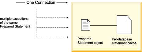
Avoiding compiling SQL statements
When you submit an SQL statement to Derby, Derby compiles and then executes the statement. Compilation is a time-consuming process that involves several steps, including optimization, the stage in which Derby makes its statement execution plan. A statement execution plan includes whether to use an index, the join order, and so on.
Unless there are significant changes in the amount of data in a table or new or deleted indexes, Derby will probably come up with the same statement execution plan for the same statement if you submit it more than once. This means that the same statements should share the same plan, and Derby should not recompile them. Derby allows you to ensure this in the following ways (in order of importance):
Using the statement cache
The statement cache is enabled by default. You can use it to avoid extra compilation overhead:
 
Your application can use PreparedStatements instead of Statements.
PreparedStatements are JDBC objects that you prepare (compile) once and execute multiple times. See the figure below. If your application executes statements that are almost but not exactly alike, use PreparedStatements, which can contain dynamic or IN parameters. Instead of using the literals for changing parameters, use question marks (?) as placeholders for such parameters. Provide the values when you execute the statement.
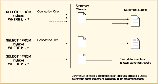
Derby supports the ParameterMetaData interface, new in JDBC 3.0. This interface describes the number, type, and properties of prepared statement parameters. See the Java DB Developer's Guide for more information.
Figure 1. A connection need only compile a PreparedStatement once
Subsequent executions can use the same statement execution plan even if the parameter values are different. (PreparedStatements are not shared across connections.)
 
 
Even if your statement uses Statements instead of PreparedStatements, Derby can reuse the statement execution plan for the statements from the statement cache. Statements from any connection can share the same statement execution plan, avoiding compilation, by using the single-statement cache. The statement cache maintains statement plans across connections. It does not, however, maintain them across reboots. See the figure below.
When, in the same database, an application submits an SQL Statement that exactly matches one already in the cache, Derby grabs the statement from the cache, even if the Statement has already been closed by the application.
To match exactly with a statement already in the cache, the SQL Statement must meet the following requirements:
 
The text must match exactly
 
The current schema must match
 
The Unicode flag that the statement was compiled under must match the current connection's flag
Remember: If your application executes statements that are almost but not exactly alike, it is more efficient to use PreparedStatements with dynamic or IN parameters.
Figure 2. A database can reuse a statement execution plan when the SQL text matches a prior statement exactly
(PreparedStatements are much more efficient.)
 
Shielding users from Derby class-loading events
JVMs tend to load classes as they are needed, which means the first time you need a class in a piece of software, it takes longer to use.
Derby has three clear cases when a lot of class loading occurs:
 
When the system boots
The system boots when you load the embedded driver, org.apache.derby.jdbc.EmbeddedDriver. In a server framework, the system boots when you start the server framework. Booting Derby loads basic Derby classes.
 
When the first database boots
Booting the first database loads some more Derby classes. The default behavior is that the first database boots when the first connection is made to it. You can also configure the system to boot databases at startup. Depending on your application, one or the other might be preferable.
 
When you compile the first query
Compiling the first query loads additional classes.
For any of these events, you can control the impact they have on users by starting them in separate threads while other tasks are occurring.
In addition, if you are using PreparedStatements, prepare them in a separate thread in the background while other tasks are occurring.
Tuning tips for multi-user systems
 
For concurrency, use row-level locking and the READ_COMMITTED isolation level.
 
For read-only applications, use table-level locking and the READ_COMMITTED isolation level.
 
Boot databases at startup to minimize the impact of connecting.
Tuning tips for single-user systems
 
Derby boots when you first load the embedded JDBC driver (org.apache.derby.jdbc.EmbeddedDriver). Load this driver during the least time-sensitive portion of your program, such as when it is booting or when you are waiting for user input. For server frameworks, the driver is loaded automatically when the server boots.
 
Boot the database at connection (the default behavior), not at startup. Connect in a background thread if possible.
 
Turn off row-level locking and use READ_COMMITTED isolation level.
Analyzing statement execution
After you create indexes, make sure that Derby is using them. In addition, you might also want to find out the join order Derby is choosing.
A general plan of attack for analyzing your application's SQL statements:
1.
 
Collect your application's most frequently used SQL statements and transactions into a single test.
2.
 
Create a benchmark test suite against which to run the sample queries. The first thing the test suite should do is checkpoint data (force Derby to flush data to disk). You can do that with the following JDBC code:
CallableStatement cs = conn.prepareCall ("CALL SYSCS_UTIL.SYSCS_CHECKPOINT_DATABASE()"); cs.execute(); cs.close();
3.
 
Use performance timings to identify poorly performing queries. Try to distinguish between cached and uncached data. Focus on measuring operations on uncached data (data not already in memory). For example, the first time you run a query, Derby returns uncached data. If you run the same query immediately afterward, Derby is probably returning cached data. The performance of these two otherwise identical statements varies significantly and skews results.
4.
 
Use RunTimeStatistics to identify tables that are scanned excessively. Check that the appropriate indexes are being used to satisfy the query and that Derby is choosing the best join order. You can also set derby.language.logQueryPlan to true to check whether indexes are being used or not. This property will is print query plans in the derby.log file. See the "Derby properties" section of the Java DB Reference Manual for details on this property. See Working with RunTimeStatistics for more information.
5.
 
Make any necessary changes and then repeat.
6.
 
If changing data access does not create significant improvements, consider other database design changes, such as denormalizing data to reduce the number of joins required. Then review the tips in Application and database design issues.
Working with RunTimeStatistics
Derby provides a language-level tool for evaluating the performance and the execution plans of statements, the RUNTIMESTATISTICS attribute.
Overview
When RUNTIMESTATISTICS is turned on for a connection, Derby maintains information about the execution plan for each statement executed within the connection (except for COMMIT) until the attribute is turned off.
For the most recently executed query, RUNTIMESTATISTICS returns information about:
 
the length of the compile time and the execute time.
This can help in benchmarking queries.
 
the statement execution plan.
This is a description of result set nodes, whether an index was used, what the join order was, how many rows qualified at each node, and how much time was spent in each node. This information can help you determine whether you need to add indexes or rewrite queries.
The exact details presented, as well as the format of presentation, can change. There are two techniques for retrieving the RUNTIMESTATISTICS information:
 
call SYSCS_UTIL.SYSCS_GET_RUNTIMESTATISTICS, which retrieves the RUNTIMESTATISTICS information as formatted text
 
call SYSCS_UTIL.SYSCS_SET_XPLAIN_SCHEMA before executing your statements, which causes Derby to store the RUNTIMESTATISTICS information in the SYSXPLAIN database tables, which can then be queried later to retrieve the data.
How you use the RUNTIMESTATISTICS attribute
 
To use the RUNTIMESTATISTICS attribute in ij, turn on and off RUNTIMESTATISTICS using the SYSCS_UTIL.SYSCS_SET_RUNTIMESTATISTICS() system procedure (see the Java DB Reference Manual for more information):
-- turn on RUNTIMESTATISTICS for connection: CALL SYSCS_UTIL.SYSCS_SET_RUNTIMESTATISTICS(1); -- execute complex query here -- step through the result set -- access runtime statistics information: VALUES SYSCS_UTIL.SYSCS_GET_RUNTIMESTATISTICS(); CALL SYSCS_UTIL.SYSCS_SET_RUNTIMESTATISTICS(0);
 
Turn on statistics timing using the SYSCS_UTIL.SYSCS_SET_STATISTICS_TIMING system procedure (see the Java DB Reference Manual for more information). If you do not turn on statistics timing, you will see the statement execution plan only, and not the timing information.
CALL SYSCS_UTIL.SYSCS_SET_RUNTIMESTATISTICS(1); CALL SYSCS_UTIL.SYSCS_SET_STATISTICS_TIMING(1);
Although the syntax is different, the basic steps for working with RUNTIMESTATISTICS are the same in a Java program.
If you are working in ij, set the display width to 5000 or another high number:
MaximumDisplayWidth 5000
Analyzing the information
Statistics timing
If you are using statistics timing, RUNTIMESTATISTICS provides information about how long each stage of the statement took. An SQL statement has two basic stages within Derby: compilation and execution. Compilation is the work done while the statement is prepared. Compilation is composed of the following stages: parsing, binding, optimization, and code generation. Execution is the actual evaluation of the statement.
Statement execution plan
RUNTIMESTATISTICS also provides information about the statement execution plan. The statement execution plan shows how long each node took to evaluate, how many rows were retrieved, whether an index was used, and so on. If an index was used, it shows the start and stop positions for the matching index scan. Looking at the plan can help you determine whether to add an index or to rewrite the query.
A statement execution plan is composed of a tree of result set nodes. A result set node represents the evaluation of one portion of the statement; it returns rows to a calling (or parent) node and can receive rows from a child node. A node can have one or more children. Starting from the top, if a node has children, it requests rows from the children. Usually only the execution plans of DML statements (queries, inserts, updates, and deletes, not dictionary object creation) are composed of more than one node.
For example, consider the following query:
SELECT * FROM Countries
This simple query involves one node only-reading all the data out of the Countries table. It involves a single node with no children. This result set node is called a Table Scan ResultSet. RUNTIMESTATISTICS text for this node looks something like this:
Statement Name: null Statement Text: select * from countries Parse Time: 20 Bind Time: 10 Optimize Time: 50 Generate Time: 20 Compile Time: 100 Execute Time: 10 Begin Compilation Timestamp : 2005-05-25 09:16:21.24 End Compilation Timestamp : 2005-05-25 09:16:21.34 Begin Execution Timestamp : 2005-05-25 09:16:21.35 End Execution Timestamp : 2005-05-25 09:16:21.4 Statement Execution Plan Text: Table Scan ResultSet for COUNTRIES at read committed isolation level using instntaneous share row locking chosen by the optimizer Number of opens = 1 Rows seen = 114 Rows filtered = 0 Fetch Size = 16 constructor time (milliseconds) = 0 open time (milliseconds) = 0 next time (milliseconds) = 10 close time (milliseconds) = 0 next time in milliseconds/row = 0 scan information: Bit set of columns fetched=All Number of columns fetched=3 Number of pages visited=3 Number of rows qualified=114 Number of rows visited=114 Scan type=heap start position: null stop position: null qualifiers: None optimizer estimated row count: 119.00 optimizer estimated cost: 69.35
Consider this second, more complex query:
SELECT Country FROM Countries WHERE Region = 'Central America'
When executed, this query involves two nodes- one to retrieve qualifying rows (the restriction is done at this node) and one to project the requested columns. So, at bottom, there is a TableScanResultSet for scanning the table. The qualifier (Region = 'Central America') is evaluated in this node. These data are passed up to the parent node, called a Project-Restrict ResultSet, in which the rows are projected-only the country column is needed (the first column in the table). RUNTIMESTATISTICS text for these two nodes looks something like this:
Statement Name: null Statement Text: SELECT Country FROM Countries WHERE Region = 'Central America' Parse Time: 10 Bind Time: 0 Optimize Time: 370 Generate Time: 10 Compile Time: 390 Execute Time: 0 Begin Compilation Timestamp : 2005-05-25 09:20:41.274 End Compilation Timestamp : 2005-05-25 09:20:41.664 Begin Execution Timestamp : 2005-05-25 09:20:41.674 End Execution Timestamp : 2005-05-25 09:20:41.674 Statement Execution Plan Text: Project-Restrict ResultSet (2): Number of opens = 1 Rows seen = 6 Rows filtered = 0 restriction = false projection = true constructor time (milliseconds) = 0 open time (milliseconds) = 0 next time (milliseconds) = 0 close time (milliseconds) = 0 restriction time (milliseconds) = 0 projection time (milliseconds) = 0 optimizer estimated row count: 11.90 optimizer estimated cost: 69.35 Source result set: Table Scan ResultSet for COUNTRIES at read committed isolation level using instantaneous share row locking chosen by the optimizer Number of opens = 1 Rows seen = 6 Rows filtered = 0 Fetch Size = 16 constructor time (milliseconds) = 0 open time (milliseconds) = 10 next time (milliseconds) = 0 close time (milliseconds) = 0 next time in milliseconds/row = 0 scan information: Bit set of columns fetched={0, 2} Number of columns fetched=2 Number of pages visited=3 Number of rows qualified=6 Number of rows visited=114 Scan type=heap start position: null stop position: null qualifiers: Column[0][0] Id: 2 Operator: = Ordered nulls: false Unknown return value: false Negate comparison result: false optimizer estimated row count: 11.90 optimizer estimated cost: 69.35
Other, more complex queries such as joins and unions have other types of result set nodes.
For inserts, updates, and deletes, rows flow out of the top, where they are inserted, updated, or deleted. For selects (queries), rows flow out of the top into a result set that is returned to the user.
The Java DB Reference Manual shows the many possible ResultSet nodes that might appear in an execution plan.
In addition, read DML statements and performance, for more information about some of the ways in which Derby executes statements.
Optimizer estimates
RUNTIMESTATISTICS show the optimizer estimates for a particular node. They show the optimizer's estimated row count and the optimizer's "estimated cost."
The estimated row count is the query optimizer's estimate of the number of qualifying rows for the table or index for the entire life of the query. If the table is the inner table of a join, the estimated row count will be for all the scans of the table, not just for a single scan of the table.
The estimated cost consists of a number, which is a relative number; it does not correspond directly to any time estimate. It is not, for example, the number of milliseconds or rows. Instead, the optimizer constructs this number for each possible access path. It compares the numbers and chooses the access path with the smallest number.
Optimizer overrides
RUNTIMESTATISTICS provides information about user-specified optimizer hints that were specified by using a -- DERBY-PROPERTIES clause.
The following example shows a SELECT statement in which the optimizer was forced to use a particular index:
SELECT * FROM t1 -- DERBY-PROPERTIES index = t1_c1 FOR UPDATE OF c2, c1
RUNTIMESTATISTICS returns the following information about this statement:
Statement Name: null Statement Text: select * from t1 --DERBY-PROPERTIES index = t1_c1 for update of c2, c1 Parse Time: 0 Bind Time: 0 Optimize Time: 0 Generate Time: 0 Compile Time: 0 Execute Time: 0 Begin Compilation Timestamp : null End Compilation Timestamp : null Begin Execution Timestamp : null End Execution Timestamp : null Statement Execution Plan Text: Index Row to Base Row ResultSet for T1: Number of opens = 1 Rows seen = 4 Columns accessed from heap = {0, 1, 2} constructor time (milliseconds) = 0 open time (milliseconds) = 0 next time (milliseconds) = 0 close time (milliseconds) = 0 User supplied optimizer overrides on T1 are { index=T1_C1 } Index Scan ResultSet for T1 using index T1_C1 at read committed isolation level using exclusive row locking chosen by the optimizer Number of opens = 1 Rows seen = 4 Rows filtered = 0 Fetch Size = 1 constructor time (milliseconds) = 0 open time (milliseconds) = 0 next time (milliseconds) = 0 close time (milliseconds) = 0 next time in milliseconds/row = 0 scan information: Bit set of columns fetched=All Number of columns fetched=2 Number of deleted rows visited=0 Number of pages visited=1 Number of rows qualified=4 Number of rows visited=4 Scan type=btree Tree height=1 start position: None stop position: None qualifiers: None
DML statements and performance
Performance and optimization
A DBMS often has a choice about the access path for retrieving data. For example, the DBMS can use an index (fast lookup for specific entries) or scan the entire table to retrieve the appropriate rows. In addition, in statements in which two tables are joined, the DBMS can choose which table to examine first (join order) and how to join the tables (join strategy). Optimization means that DBMS makes the best (optimal) choice of access paths, join order, and join strategy. True query optimization means that the DBMS will usually make a good choice regardless of how the query is written. The optimizer does not necessarily make the best choice, just a good one.
Derby can use indexes to improve the performance of DML (data manipulation language) statements such as queries, updates, and deletes. The query optimizer can make decisions about whether to use an index for a particular table (access path) and also makes decisions about join order, type of join, and a few other matters.
This section gives an overview of the Derby optimizer and discusses performance issues in the execution of DML statements.
Index use and access paths
If you define an index on a column or columns, the query optimizer can use the index to find data in the column more quickly. Derby automatically creates indexes to back up primary key, foreign key, and unique constraints, so those indexes are always available to the optimizer, as well as those that you explicitly create with the CREATE INDEX command. The way Derby gets to the data-via an index or directly via the table-is called the access path.
What is an index?
An index is a database structure that provides quick lookup of data in a column or columns of a table.
For example, a Flights table in a travelDB database has three indexes:
 
An index on the orig_airport column (called OrigIndex)
 
An index on the dest_airport column (called DestIndex)
 
An index enforcing the primary key constraint on the flight_id and segment_number columns (which has a system-generated name)
This means there are three separate structures that provide shortcuts into the Flights table. Let's look at one of those structures, OrigIndex.
OrigIndex stores every value in the orig_airport column, plus information on how to retrieve the entire corresponding row for each value.
 
For every row in Flights, there is an entry in OrigIndex that includes the value of the orig_airport column and the address of the row itself. The entries are stored in ascending order by the orig_airport values.
When an index includes more than one column, the first column is the main one by which the entries are ordered. For example, the index on (flight_id, segment_number) is ordered first by flight_id. If there is more than one flight_id of the same value, those entries are then ordered by segment_number. An excerpt from the entries in the index might look like this:
'AA1111' 1 'AA1111' 2 'AA1112' 1 'AA1113' 1 'AA1113' 2
Indexes are helpful only sometimes. This particular index is useful when a statement's WHERE clause is looking for rows for which the value of orig_airport is some specific value or range of values. SELECTs, UPDATEs, and DELETEs can all have WHERE clauses.
For example, OrigIndex is helpful for statements such as the following:
SELECT * FROM Flights WHERE orig_airport = 'SFO' SELECT * FROM Flights WHERE orig_airport < 'BBB' SELECT * FROM Flights WHERE orig_airport >= 'MMM'
DestIndex is helpful for statements such as the following:
SELECT * FROM Flights WHERE dest_airport = 'SCL'
The primary key index (on flight_id and segment_number) is helpful for statements such as the following:
SELECT * FROM Flights WHERE flight_id = 'AA1111' SELECT * FROM Flights WHERE flight_id BETWEEN 'AA1111' AND 'AA1115' SELECT * FROM FlightAvailability AS fa, Flights AS fts WHERE flight_date > CURRENT_DATE AND fts.flight_id = fa.flight_id AND fts.segment_number = fa.segment_number
The next section discusses why the indexes are helpful for these statements but not for others.
What's optimizable?
As you learned in the previous section, Derby might be able to use an index on a column to find data more quickly. If Derby can use an index for a statement, that statement is said to be optimizable. The statements shown in the preceding section allow Derby to use the index because their WHERE clauses provide start and stop conditions. That is, they tell Derby the point at which to begin its scan of the index and where to end the scan.
For example, a statement with a WHERE clause looking for rows for which the orig_airport value is less than BBB means that Derby must begin the scan at the beginning of the index; it can end the scan at BBB. This means that it avoids scanning the index for most of the entries.
An index scan that uses start or stop conditions is called a matching index scan.
Note: A WHERE clause can have more than one part. Parts are linked with the word AND or OR. Each part is called a predicate. WHERE clauses with predicates joined by OR are not optimizable. WHERE clauses with predicates joined by AND are optimizable if at least one of the predicates is optimizable. For example:
SELECT * FROM Flights WHERE flight_id = 'AA1111' AND segment_number <> 2
In this example, the first predicate is optimizable; the second predicate is not. Therefore, the statement is optimizable.
Note: In a few cases, a WHERE clause with predicates joined by OR can be transformed into an optimizable statement. See OR transformations.
Directly optimizable predicates:
Some predicates provide clear-cut starting and stopping points. A predicate provides start or stop conditions, and is therefore optimizable, when:
 
It uses a simple column reference to a column (the name of the column, not the name of the column within an expression or method call). For example, the following is a simple column reference:
WHERE orig_airport = 'SFO'
The following is not:
WHERE lower(orig_airport) = 'sfo'
 
It refers to a column that is the first or only column in the index.
References to contiguous columns in other predicates in the statement when there is a multi-column index can further define the starting or stopping points. (If the columns are not contiguous with the first column, they are not optimizable predicates but can be used as qualifiers.) For example, given a composite index on FlightAvailability (flight_id, segment_number, and flight_date), the following predicate satisfies that condition:
WHERE flight_id = 'AA1200' AND segment_number = 2
The following one does not:
WHERE flight_id = 'AA1200' AND flight_date = CURRENT_DATE
 
The column is compared to a constant or to an expression that does not include columns in the same table. Examples of valid expressions: other_table.column_a, ? (dynamic parameter), 7+9. The comparison must use the following operators:
 
=
 
<
 
<=
 
>
 
>=
 
IS NULL
Indirectly optimizable predicates:
Some predicates are transformed internally into ones that provide starting and stopping points and are therefore optimizable.
Predicates that use the following comparison operators can be transformed internally into optimizable predicates:
 
BETWEEN
 
LIKE (in certain situations)
 
IN (in certain situations)
For details on these and other transformations, see Internal language transformations.
Joins:
Joins specified by the JOIN keyword are optimizable. This means that Derby can use an index on the inner table of the join (start and stop conditions are being supplied implicitly by the rows in the outer table).
Note that joins built using traditional predicates are also optimizable. For example, the following statement is optimizable:
SELECT * FROM Countries, Cities WHERE Countries.country_ISO_code = Cities.country_ISO_code
Covering indexes
Even when there is no definite starting or stopping point for an index scan, an index can speed up the execution of a query if the index covers the query. An index covers the query if all the columns specified in the query are part of the index. These are the columns that are all columns referenced in the query, not just columns in a WHERE clause. If so, Derby never has to go to the data pages at all, but can retrieve all data through index access alone. For example, in the following queries, OrigIndex covers the query:
SELECT orig_airport FROM Flights SELECT DISTINCT lower(orig_airport) FROM Flights FROM Flights
Derby can get all required data out of the index instead of from the table.
Note: If the query produces an updatable result set, Derby will retrieve all data from the data pages even if there is an index that covers the query.
Single-column index examples:
The following queries do not provide start and stop conditions for a scan of OrigIndex, the index on the orig_airport column in Flights. However, some of these queries allow Derby to do an index rather than a table scan because the index covers the query.
-- Derby would scan entire table; comparison is not with a -- constant or with a column in another table SELECT * FROM Flights WHERE orig_airport = dest_airport -- Derby would scan entire table; <> operator is not optimizable SELECT * FROM Flights WHERE orig_airport <> 'SFO' -- not valid operator for matching index scan -- However, Derby would do an index -- rather than a table scan because -- index covers query SELECT orig_airport FROM Flights WHERE orig_airport <> 'SFO' -- use of a function is not simple column reference -- Derby would scan entire index, but not table -- (index covers query) SELECT orig_airport FROM Flights WHERE lower(orig_airport) = 'sfo'
Multiple-column index example:
The following queries do provide start and stop conditions for a scan of the primary key index on the flight_id and segment_number columns in Flights:
-- the where clause compares both columns with valid -- operators to constants SELECT * FROM Flights WHERE flight_id = 'AA1115' AND segment_number < 2 -- the first column is in a valid comparison SELECT * FROM Flights WHERE flight_id < 'BB' -- LIKE is transformed into >= and <=, providing -- start and stop conditions SELECT * FROM Flights WHERE flight_id LIKE 'AA%'
The following queries do not:
-- segment_number is in the index, but it's not the first column; -- there's no logical starting and stopping place SELECT * FROM Flights WHERE segment_number = 2 -- Derby would scan entire table; comparison of first column -- is not with a constant or column in another table -- and no covering index applies SELECT * FROM Flights WHERE orig_airport = dest_airport AND segment_number < 2
Useful indexes can use qualifiers
Matching index scans can use qualifiers that further restrict the result set. Remember that a WHERE clause that contains at least one optimizable predicate is optimizable. Nonoptimizable predicates can be useful in other ways.
Consider the following query:
SELECT * FROM FLIGHTS WHERE orig_airport < 'BBB' AND orig_airport <> 'AKL'
The second predicate is not optimizable, but the first predicate is. The second predicate becomes a qualification for which Derby evaluates the entries in the index as it traverses it.
 
The following comparisons are valid qualifiers:
 
=
 
<
 
<=
 
>
 
>=
 
IS NULL
 
BETWEEN
 
LIKE
 
<>
 
IS NOT NULL
 
The qualifier's reference to the column does not have to be a simple column reference; you can put the column in an expression.
 
The qualifier's column does not have to be the first column in the index and does not have to be contiguous with the first column in the index.
When a table scan Is better
Sometimes a table scan is the most efficient way to access data, even if a potentially useful index is available. For example, if the statement returns virtually all the data in the table, it is more efficient to go straight to the table instead of looking values up in an index, because then Derby is able to avoid the intermediate step of retrieving the rows from the index lookup values.
For example:
SELECT * FROM Flights WHERE dest_airport < 'Z'
In the Flights table, most of the airport codes begin with letters that are less than Z. Depending on the number of rows in the table, it is probably more efficient for Derby to go straight to the table to retrieve the appropriate rows. However, for the following query, Derby uses the index:
SELECT * FROM Flights WHERE dest_airport < 'B'
Only a few flights have airport codes that begin with a letter less than B.
Indexes have a cost for inserts, updates, and deletes
Derby has to do work to maintain indexes. If you insert into or delete from a table, the system has to insert or delete rows in all the indexes on the table. If you update a table, the system has to maintain those indexes that are on the columns being updated. So having a lot of indexes can speed up select statements, but slow down inserts, updates, and deletes.
Note: Updates and deletes with WHERE clauses can use indexes for scans, even if the indexed column is being updated.
Joins and performance
Joins, SQL statements in which Derby selects data from two or more tables using one or more key columns from each table, can vary widely in performance. Factors that affect the performance of joins are join order, indexes, and join strategy.
Join order overview
The Derby optimizer usually makes a good choice about join order. This section discusses the performance implications of join order.
In a join operation involving two tables, Derby scans the tables in a particular order. Derby accesses rows in one table first, and this table is now called the outer table.
Then, for each qualifying row in the outer table, Derby looks for matching rows in the second table, which is called the inner table.
Derby accesses the outer table once, and the inner table probably many times (depending on how many rows in the outer table qualify).
This leads to a few general rules of thumb about join order:
 
If the join has no restrictions in the WHERE clause that would limit the number of rows returned from one of the tables to just a few, the following rules apply:
 
If only one table has an index on the joined column or columns, it is much better for that table to be the inner table. This is because for each of the many inner table lookups, Derby can use an index instead of scanning the entire table.
 
Since indexes on inner tables are accessed many times, if the index on one table is smaller than the index on another, the table with the smaller one should probably be the inner table. That is because smaller indexes (or tables) can be cached (kept in Derby's memory, allowing Derby to avoid expensive I/O for each iteration).
 
On the other hand, if a query has restrictions in the WHERE clause for one table that would cause it to return only a few rows from that table (for example, WHERE flight_id = 'AA1111'), it is better for the restricted table to be the outer table. Derby will have to go to the inner table only a few times anyway.
Consider:
SELECT * FROM huge_table, small_table WHERE huge_table.unique_column = 1 AND huge_table.other_column = small_table.non_unique_column
 
In this case, the qualification huge_table.unique_column = 1 (assuming a unique index on the column) qualifies only one row, so it is better for huge_table to be the outer table in the join.
Join strategies
The most common join strategy in Derby is called a nested loop. For each qualifying row in the outer table, Derby uses the appropriate access path (index or table) to find the matching rows in the inner table.
Another type of join in Derby is called a hash join. For joins of this type, Derby constructs a hash table representing all the selected columns of the inner table. For each qualifying row in the outer table, Derby does a quick lookup on the hash table to get the inner table data. Derby has to scan the inner table or index only once, to build the hash table.
Nested loop joins are preferable in most situations.
Hash joins are preferable in situations in which the inner table values are unique and there are many qualifying rows in the outer table. Hash joins require that the statement's WHERE clause be an optimizable equijoin:
 
It must use the = operator to compare column(s) in the outer table to column(s) in the inner table.
 
References to columns in the inner table must be simple column references. Simple column references are described in Directly optimizable predicates.
The hash table for a hash join is held in memory and if it gets big enough, it will spill to the disk. The optimizer makes a very rough estimate of the amount of memory required to make the hash table. If it estimates that the amount of memory required would exceed the system-wide limit of memory use for a table, the optimizer chooses a nested loop join instead.
If memory use is not a problem for your environment, set this property to a high number; allowing the optimizer the maximum flexibility in considering a join strategy queries involving large queries leads to better performance. It can also be set to smaller values for more limited environments.
Note: Derby allows multiple columns as hash keys.
Derby's cost-based optimization
The query optimizer makes cost-based decisions to determine:
 
Which index (if any) to use on each table in a query (see About the optimizer's choice of access path)


Whether to avoid additional sorting (see About the optimizer's choice of sort avoidance)
 
Automatic lock escalation (see About the system's selection of lock granularity)
 
Whether to use bulk fetch (see About the optimizer's selection of bulk fetch)
About the optimizer's choice of access path
The optimizer's choice of access path can depend on the number of rows it will have to read. It tries to choose a path that requires the fewest number of rows read. For joins, the number of rows read also depends heavily on the join order (discussed in About the optimizer's choice of join order.)
How does the optimizer know how many rows a particular access path will read? The answer: sometimes it knows exactly, and sometimes it has to make an educated guess. See Selectivity and cardinality statistics.
About the optimizer's choice of join order
The optimizer chooses the optimal join order as well as the optimal index for each table. The join order can affect which index is the best choice. The optimizer can choose an index as the access path for a table if it is the inner table, but not if it is the outer table (and there are no further qualifications).
The optimizer chooses the join order of tables only in simple FROM clauses. Most joins using the JOIN keyword are flattened into simple joins, so the optimizer chooses their join order.
The optimizer does not choose the join order for outer joins; it uses the order specified in the statement.
When selecting a join order, the optimizer takes into account:
 
The size of each table
 
The indexes available on each table
 
Whether an index on a table is useful in a particular join order
 
The number of rows and pages to be scanned for each table in each join order
Note: Derby does transitive closure on qualifications. For details, see Transitive closure.
Join order case study:
For example, consider the following situation:
The Flights table (as you know) stores information about flight segments. It has a primary key on the flight_id and segment_number columns. This primary key constraint is backed up by a unique index on those columns.
The FlightAvailability table, which stores information about the availability of flight segments on particular days, can store several rows for a particular row in the Flights table (one for each date).
You want to see information about all the flights, and you issue the following query:
SELECT * FROM FlightAvailability AS fa, Flights AS fts WHERE fa.flight_id = fts.flight_id AND fa.segment_number = fts.segment_number
First imagine the situation in which there are no useful indexes on the FlightAvailability table.
Using the join order with FlightAvailability as the outer table and Flights as the inner table is cheaper because it allows the flight_id/segment_number columns from FlightAvailability to be used to probe into and find matching rows in Flights, using the primary key index on Flights.flight_id and Flights.segment_number.
This is preferable to the opposite join order (with Flights as the outer table and FlightAvailability as the inner table) because in that case, for each row in Flights, the system would have to scan the entire FlightAvailability table to find the matching rows (because there is no useful index- an index on the flight_id/segment_number columns).
Second, imagine the situation in which there is a useful index on the FlightAvailability table (this is actually the case in the sample database). FlightAvailability has a primary key index on flight_id, segment_number, and booking_date. In that index, the flight_id-segment_number combination is not unique, since there is a one-to-many correspondence between the Flights table and the FlightAvailability table. However, the index is still very useful for finding rows with particular flight_id/segment_number values.
You issue the same query:
SELECT * FROM FlightAvailability AS fa, Flights AS fts WHERE fa.flight_id = fts.flight_id AND fa.segment_number = fts.segment_number
Although the difference in cost is smaller, it is still cheaper for the Flights table to be the inner table, because its index is unique, whereas FlightAvailability's index is not. That is because it is cheaper for Derby to step through a unique index than through a non-unique index.
About the optimizer's choice of join strategy
The optimizer compares the cost of choosing a hash join (if a hash join is possible) to the cost of choosing a nested loop join and chooses the cheaper strategy. For information about when hash joins are possible, see Join strategies.
In some cases, the size of the hash table that Derby would have to build is prohibitive and can cause the JVM to run out of memory. For this reason, the optimizer has an upper limit on the size of a table on which it will consider a hash join. It will not consider a hash join for a statement if it estimates that the size of the hash table would exceed the system-wide limit of memory use for a table, the optimizer chooses a nested loop join instead. The optimizer's estimates of size of hash tables are approximate only.
About the optimizer's choice of sort avoidance
Some SQL statements require that data be ordered, including those with ORDER BY, GROUP BY, and DISTINCT. MIN() and MAX() aggregates also require ordering of data.
Derby can sometimes avoid sorting steps for:
 
statements with ORDER BY
Derby can also perform the following optimizations, but they are not based on cost:
 
sort avoidance for DISTINCT and GROUP BYs
 
statements with a MIN() aggregate
Cost-based ORDER BY sort avoidance:
Usually, sorting requires an extra step to put the data into the right order. This extra step can be avoided for data that are already in the right order. For example, if a single-table query has an ORDER BY on a single column, and there is an index on that column, sorting can be avoided if Derby uses the index as the access path.
Where possible, Derby's query compiler transforms an SQL statement internally into one that avoids this extra step. For information about internal transformations, see Sort avoidance. This transformation, if it occurs, happens before optimization. After any such transformations are made, the optimizer can do its part to help avoid a separate sorting step by choosing an already sorted access path. It compares the cost of using that path with the cost of sorting. Derby does this for statements that use an ORDER BY clause in the following situations:
 
The statements involve tables with indexes that are in the correct order.
 
The statements involve scans of unique indexes that are guaranteed to return only one row per scan.
ORDER BY specifies a priority of ordering of columns in a result set. For example, ORDER BY X, Y means that column X has a more significant ordering than column Y.
The situations that allow Derby to avoid a separate ordering step for statements with ORDER BY clauses are:
 
Index scans, which provide the correct order.
-- covering index SELECT flight_id FROM Flights ORDER BY flight_id
 
The rows from a table when fetched through an index scan.
-- if Derby uses the index on orig_airport -- to access the data, it can avoid the sort -- required by the final ORDER BY SELECT orig_airport, miles FROM FLIGHTS WHERE orig_airport < 'DDD' ORDER BY orig_airport
 
The rows from a join when ordered by the indexed column or columns in the outer table.
-- if Derby chooses Cities as the outer table, it -- can avoid a separate sorting step SELECT * FROM cities, countries WHERE cities.country_ISO_code = countries.country_ISO_code AND cities.country_ISO_code < 'DD' ORDER BY cities.country_ISO_code
 
Result sets that are guaranteed to return a single row. They are ordered on all of their columns (for example, if there are equality conditions on all the columns in a unique index, all the columns returned for that table can be considered ordered, with any priority of ordering of the columns).
-- query will only return one row, so that row is -- "in order" for ANY column SELECT miles FROM Flights WHERE flight_id = 'US1381' AND segment_number = 2 ORDER BY miles
 
Any column in a result set that has an equality comparison with a constant. The column is considered ordered with no priority to its ordering.
-- The comparison of segment_number -- to a constant means that it is always correctly -- ordered. Using the index on (flight_id, segment_number) -- as the access path means -- that the ordering will be correct for the ORDER BY -- clause in this query. The same thing would be true if -- flight_id were compared to a constant instead. SELECT segment_number, flight_id FROM Flights WHERE segment_number=2 ORDER BY segment_number, flight_id
And because of transitive closure, this means that even more complex statements can avoid sorting. For example:
-- transitive closure means that Derby will -- add this clause: -- AND countries.country_ISO_code = 'CL', which means -- that the ordering column is now compared to a constant, -- and sorting can be avoided. SELECT * FROM cities, countries WHERE cities.country_ISO_code = 'CL' AND cities.country_ISO_code = countries.country_ISO_code ORDER BY countries.country_ISO_code
For more information about transitive closure and other statement transformations, see Internal language transformations.
About the system's selection of lock granularity
When a system is configured for row-level locking, it decides whether to use table-level locking or row-level locking for each table in each DML statement. The system bases this decision on the number of rows read or written for each table, and on whether a full conglomerate scan is done for each table.
Note: When you have turned off row-level locking for your system, Derby always uses table-level locking.
The first goal of the system's decision is concurrency; wherever possible, the system chooses row-level locking. However, row-level locking uses a lot of resources and might have a negative impact on performance. Sometimes row-level locking does not provide much more concurrency than table-level locking. In those situations, the system might choose to escalate the locking scheme from row-level locking to table-level locking to improve performance. For example, if a connection is configured for TRANSACTION_SERIALIZABLE isolation, the system chooses table-level locking for the following statement:
SELECT * FROM FlightAvailability AS fa, Flights AS fts WHERE fts.flight_id = fa.flight_id AND fts.segment_number = fa.segment_number
To satisfy the isolation requirements, Derby would have to lock all the rows in both the FlightAvailability and the Flights tables. Locking both the tables would be cheaper, would provide the same isolation, and would allow the same concurrency.
Note: You can force lock escalation for specific tables when you alter them with the LOCKSIZE clause. For these tables, Derby always chooses table-level locking. For more information, see the Java DB Reference Manual.
How the system makes its decision if it has a choice:
If the lock granularity (whether to lock rows or entire tables) is not forced by the user, the system makes a decision using the following rules:
 
For SELECT statements running in READ_COMMITTED isolation, the system always chooses row-level locking.
 
If the statement scans the entire table or index and it does not meet the criteria above, the system chooses table-level locking. (A statement scans the entire table whenever it chooses a table as the access path.)
 
If a statement partially scans the index, the system uses row-level locking, until the number of rows touched on a table reaches lock escalation threshold. It is then escalated to a table lock. (You can configure this threshold number; see Lock escalation threshold.)
 
For SELECT, UPDATE, and DELETE statements, the number of rows touched is different from the number of rows read. If the same row is read more than once, it is considered to have been touched only once. Each row in the inner table of a join can be read many times, but can be touched at most one time.
Lock escalation threshold:
The system property derby.locks.escalationThreshold determines the threshold for number of rows touched for a particular table above which the system will escalate to table-level locking. The default value of this property is 5000. For large systems, set this property to a higher value. For smaller systems, lower it. See the "Derby properties" section of the Java DB Reference Manual for details on this property.
This property also sets the threshold for transaction-based lock escalation (see Transaction-based lock escalation).
Note: For more information about lock escalation, see Locking and performance.
About the optimizer's selection of bulk fetch
When Derby retrieves data from a conglomerate, it can fetch more than one row at a time. Fetching more than one row at a time is called bulk fetch. By default, Derby fetches 16 rows at a time.
Bulk fetch is faster than retrieving one row at a time when a large number of rows qualify for each scan of the table or index. Bulk fetch uses extra memory to hold the pre-fetched rows, so it should be avoided in situations in which memory is scarce.
Bulk fetch is automatically turned off for updatable cursors, for hash joins, for statements in which the scan returns a single row, and for subqueries. It is useful, however, for table scans or index range scans:
SELECT * FROM Flights WHERE miles > 4 SELECT * FROM Flights
The default size for bulk fetch (16 rows) typically provides good performance.
Locking and performance
Row-level locking improves concurrency in a multi-user system. However, a large number of row locks can degrade performance. About the system's selection of lock granularity discussed the way the optimizer makes some compile-time decisions about escalating row locks to table locks for performance reasons. This section discusses ways in which the Derby system and the user can make similar lock escalations.
Transaction-based lock escalation
The optimizer makes its decisions for the scope of a single statement at compile time; the runtime overrides are also for the scope of a single statement. As you know, a transaction can span several statements. For connections running in TRANSACTION_SERIALIZABLE isolation and for connections that are doing a lot of inserts or updates, a transaction can accumulate a number of row locks even though no single statement would touch enough rows to make the optimizer choose table-level locking for any single table.
However, during a transaction, the Derby system tracks the number of locks for all tables in the transaction, and when this number exceeds a threshold number (which you can configure; see Lock escalation threshold), the system attempts to escalate locking for at least one of the tables involved from row-level to table-level locking.
The system attempts to escalate to table-level locking for each table that has a burdensome number of locks by trying to obtain the relevant table lock. If the system can lock the table without waiting, the system locks the entire table and releases all row locks for the table. If the system cannot lock the table without waiting, the system leaves the row locks intact.
After a table is locked in either mode, a transaction does not acquire any subsequent row-level locks on a table. For example, if you have a table called Hotels that contained several thousand rows and a transaction locks the entire table in share mode in order to read data, it might later need to lock a particular row in exclusive mode in order to update the row. However, the previous table-level lock on Hotels forces the exclusive lock to be table-level as well.
This transaction-based runtime decision is independent of any compilation decision.
If when the escalation threshold was exceeded the system did not obtain any table locks because it would have had to wait, the next lock escalation attempt is delayed until the number of held locks has increased by some significant amount, for example from 5000 to 6000.
Here are some examples assuming the escalation threshold is 5000:
 
Single table holding the majority of the locks
Table
Number of row locks
Promote?
Hotels
4853
yes
Countries
3
no
Cities
12
no
 
Two tables holding the majority of the locks
Table
Number of row locks
Promote?
Hotels
2349
yes
Countries
3
no
Cities
1800
yes
 
Many tables holding a small number of locks
Table
Number of row locks
Promote?
table001
279
no
table002
142
no
table003
356
no
table004
79
no
table194
384
no
table195
416
no
Locking a table for the duration of a transaction
In addition, you can explicitly lock a table for the duration of a transaction with the LOCK TABLE statement. This is useful if you know in advance that an entire table should be locked and want to save the resources required for obtaining row locks until the system escalates the locking. For information about this feature, see "LOCK TABLE statement" in the Java DB Reference Manual.
Non-cost-based optimizations
The optimizer makes some non-cost-based optimizations, which means that it does not consider them when determining the access path and join order. If all the conditions are right, it makes the optimizations after the access path and join order are determined.
Non-cost-based sort avoidance (tuple filtering)
In most cases, Derby needs to perform two separate steps for statements that use DISTINCT or GROUP BY: first sorting the selected columns, then either discarding duplicate rows or aggregating grouped rows. Sometimes it is able to avoid sorting for these statements with tuple filtering. Tuple filtering means that the rows are already in a useful order. For DISTINCT, Derby can simply filter out duplicate values when they are found and return results to the user sooner. For GROUP BY, Derby can aggregate a group of rows until a new set of rows is detected and return results to the user sooner.
These are non-cost-based optimizations; the optimizer does not yet consider the cost of these optimizations.
The examples in this section refer to the following tables:
CREATE TABLE t1(c1 INT, c2 INT, c3 INT, c4 INT) CREATE INDEX i1 ON t1(c1) CREATE INDEX i1_2_3_4 ON t1(c1, c2, c3, c4)
DISTINCT
Tuple filtering is applied for a DISTINCT when the following criteria are met:
 
The SELECT list is composed entirely of simple column references and constants.
 
All simple column references come from the same table and the optimizer has chosen the table in question to be the outermost table in the query block.
 
The optimizer has chosen an index as the access path for the table in question.
 
The simple column references in the SELECT list, plus any simple column references from the table that have equality predicates on them, are a prefix of the index that the optimizer selected as the access path for the table.
Note: The set of column references must be an in-order prefix of the index.
Here is the most common case in which tuple filtering will be applied:
SELECT DISTINCT c1 FROM t1
Equality predicates allow tuple filtering on the following:
SELECT DISTINCT c2 FROM t1 WHERE c1 = 5 SELECT DISTINCT c2, c4 FROM t1 WHERE c1 = 5 and c3 = 7 -- the columns don't have to be in the -- same order as the index SELECT DISTINCT c2, c1 FROM t1
Quick DISTINCT scans:
Derby can use a hash table instead of a sorter to eliminate duplicates when performing a DISTINCT in the following cases:
 
There is a single table in the query block.
 
An ORDER BY clause is not merged into the DISTINCT.
 
All entries in the SELECT list are simple column references.
 
There are no predicates in the query block.
This technique allows for minimal locking when performing the scan at the READ COMMITTED isolation level.
Note: This technique appears in RunTimeStatistics as a DistinctScanResultSet.
GROUP BY
Tuple filtering is applied for a GROUP BY when the following criteria are met:
 
All grouping columns come from the same table and the optimizer has chosen the table in question to be the outermost table in the query block.
 
The optimizer has chosen an index as the access path for the table in question.
 
The grouping columns, plus any simple column references from the table that have equality predicates on them, are a prefix of the index that the optimizer selected as the access path for the table.
Here is the most common case in which tuple filtering will be applied:
SELECT max(c2) FROM t1 GROUP BY c1
Equality predicates allow tuple filtering on the following:
SELECT c2, SUM(c3) FROM t1 WHERE c1 = 5 GROUP BY c2 SELECT max(c4) FROM t1 WHERE c1 = 5 AND c3 = 6 GROUP BY c2
The MIN() and MAX() optimizations
The optimizer knows that it can avoid iterating through all the source rows in a result to compute a MIN() or MAX() aggregate when data are already in the right order. When data are guaranteed to be in the right order, Derby can go immediately to the smallest (minimum) or largest (maximum) row.
The following conditions must be true:
 
The MIN() or MAX() is the only entry in the SELECT list.
 
The MIN() or MAX() is on a simple column reference, not on an expression.
 
For MAX(), there must not be a WHERE clause.
 
For MIN():
 
The referenced table is the outermost table in the optimizer's chosen join order for the query block.
 
The optimizer chose an index containing the referenced column as the access path.
 
The referenced column is the first key column in that index OR the referenced column is a key column in that index and equality predicates exist on all key columns prior to the simple column reference in that index.
For example, the optimizer can use this optimization for the following queries (if the optimizer uses the appropriate indexes as the access paths):
-- index on orig_airport SELECT MIN(orig_airport) FROM Flights -- index on orig_airport SELECT MAX(orig_airport) FROM Flights -- index on orig_airport SELECT miles FROM Flights WHERE orig_airport = (SELECT MIN(orig_airport) FROM Flights) -- index on segment_number, flight_id SELECT MIN(segment_number) FROM Flights WHERE flight_id = 'AA1111' SELECT * FROM Flights WHERE segment_number = (SELECT MIN(segment_number) FROM Flights WHERE flight_id = 'AA1111')
The optimizer decides whether to implement the optimization after choosing the plan for the query. The optimizer does not take this optimization into account when costing the plan.
Overriding the default optimizer behavior
You can override the default behavior of the Derby query optimizer by including a --DERBY-PROPERTIES clause and an associated property as a comment within an SQL statement.
Because optimizer overrides are expressed as comments, they must be included at the end of a line. You can specify optimizer override properties for an entire FROM clause, for tables in the FROM clause, or for both.
The syntax for a FROM clause property is:
FROM [ -- DERBY-PROPERTIES joinOrder = { FIXED | UNFIXED } ]         TableExpression [,TableExpression]*
The syntax for table optimizer override properties, which must be included at the end of a TableExpression, is:
{table-Name | view-Name }         [ [ AS ] correlation-Name          [ (Simple-column-Name [ , Simple-column-Name ]* ) ] ]         [ -- DERBY-PROPERTIES { constraint = constraint-Name | index = index-Name | joinStrategy = { NESTEDLOOP | HASH } } ]
The space between -- and DERBY-PROPERTIES is optional.
> Important: Make sure that you adhere to the correct syntax when using the --DERBY-PROPERTIES clause. Failure to do so can cause the parser to interpret it as a comment and ignore it. To verify that the parser interpreted your overrides correctly, you can use RunTimeStatistics. See Optimizer overrides for more information.
The following four properties are available for use in a --DERBY-PROPERTIES clause:
constraint
To force the use of the index that enforces a primary key, a foreign key, or unique constraint, use the constraint property and specify the unqualified name of the constraint. The constraint property can be used only within a TableExpression, and it can be specified only on base tables; it cannot be specified on views or derived tables.
index
The index property is similar to the constraint property. To force use of a particular index, specify the unqualified index name. To force a table scan, specify null for the index name. The index property can be used only within a TableExpression, and it can be specified only on base tables; it cannot be specified on views or derived tables.
joinOrder
Use the joinOrder property to override the optimizer’s choice of join order for two tables. When the value FIXED is specified, the optimizer will choose the order of tables as they appear in the FROM clause as the join order. Valid values for the joinOrder property include FIXED and UNFIXED. The joinOrder property can be used with a FROM clause.
joinStrategy
Use the joinStrategy property to override the optimizer’s choice of join strategy. The two types of join strategy are called nested loop and hash. In a nested loop join strategy, for each qualifying row in the outer table, Derby uses the appropriate access path (index or table scan) to find the matching rows in the inner table. In a hash join strategy, Derby constructs a hash table that represents the inner table. For each qualifying row in the outer table, Derby does a quick lookup on the hash table to find the matching rows in the inner table. Derby needs to scan the inner table or index only once to create the hash table. The --DERBY-PROPERTIES parameter must immediately follow the inner table.
Typically, you will use the joinStrategy property only in conjunction with the joinOrder property. Specifying a join strategy without knowing the join order can result in less-than-optimal performance.
Valid values include HASH and NESTEDLOOP. The joinStrategy property can be used only within a TableExpression.
The following examples illustrate the use of the --DERBY-PROPERTIES clause:
constraint
CREATE TABLE t1 (c1 int, c2 int, c3 int, CONSTRAINT cons1 PRIMARY KEY (c1, c2)) INSERT INTO t1 VALUES (1, 1, 1), (2, 2, 2), (3, 3, 3), (4, 4, 4) SELECT * FROM t1 --DERBY-PROPERTIES constraint=cons1 FOR UPDATE
index
CREATE TABLE t1 (c1 int, c2 int, c3 int, CONSTRAINT cons1 PRIMARY KEY (c1, c2)) INSERT INTO t1 VALUES (1, 1, 1), (2, 2, 2), (3, 3, 3), (4, 4, 4) CREATE INDEX t1_c1 ON t1(c1) SELECT * FROM t1 --DERBY-PROPERTIES index=t1_c1 WHERE c1=1
joinOrder
CREATE TABLE t1 (c1 int, c2 int, c3 int, CONSTRAINT cons1 PRIMARY KEY (c1, c2)) CREATE TABLE t2 (c1 int not null, c2 int not null, c3 int, CONSTRAINT cons2 UNIQUE (c1, c2)) INSERT INTO t1 VALUES (1, 1, 1), (2, 2, 2), (3, 3, 3), (4, 4, 4) INSERT INTO t2 VALUES (1, 1, 1), (2, 2, 2), (3, 3, 3), (4, 4, 4) SELECT * FROM --DERBY-PROPERTIES joinOrder=FIXED t1, t2 WHERE t1.c1=t2.c1
joinStrategy
CREATE TABLE t1 (c1 int, c2 int, c3 int, CONSTRAINT cons1 PRIMARY KEY (c1, c2)) CREATE TABLE t2 (c1 int not null, c2 int not null, c3 int, CONSTRAINT cons2 UNIQUE (c1, c2)) INSERT INTO t1 VALUES (1, 1, 1), (2, 2, 2), (3, 3, 3), (4, 4, 4) INSERT INTO t2 VALUES (1, 1, 1), (2, 2, 2), (3, 3, 3), (4, 4, 4) SELECT * FROM --DERBY-PROPERTIES joinOrder=FIXED t1 a, t1 b --DERBY-PROPERTIES joinStrategy=NESTEDLOOP WHERE a.c1=b.c1
Selectivity and cardinality statistics
The optimizer determines the number of rows that will be scanned from disk when deciding on an access path for a particular table (whether to use an index or to scan the table).
 
The optimizer knows "exactly" the number of rows that will be scanned from disk for table scans (see Determinations of rows scanned from disk for a table scan).
 
For index scans, the optimizer must estimate the number of rows that will be scanned from disk. (see Estimations of rows scanned from disk for an index scan). Derby might be able to use cardinality statistics to make a better estimate of the number of rows that will be scanned from disk as described in this chapter.
Determinations of rows scanned from disk for a table scan
For table scans, the optimizer does not need to estimate the number of rows that will be scanned from disk during the scan; the number of rows that will be scanned from disk will be equal to the number of rows in the table, as described below.
How the optimizer determines the number of rows in a table
The optimizer uses a stored row count to determine the number of rows in a table, which is maintained automatically by the system.
Normally, an updated value is stored in the database whenever the database goes through an orderly shutdown (as long as the database is not read-only). Stored row counts become inaccurate if there is a non-orderly shutdown (for example, a power failure or other type of system crash).
You can correct the optimizer's row count without shutting down the system; Derby sets the stored row count for a table to the correct value whenever a query that does a full scan on the base conglomerate finishes. For example, executing the following query sets the row count for table Flights to the correct value:
SELECT * FROM Flights
Derby also sets the stored row count on a table to the correct value whenever a user creates a new index or primary key, unique, or foreign key constraint on the table. This value is not guaranteed to be written to disk.
Estimations of rows scanned from disk for an index scan
When an index is available, the optimizer has to estimate the number of rows that will be scanned from disk. The accuracy of this estimate depends on the type of query being optimized.
Queries with a known search condition
When the exact start and stop conditions are known at compilation time, the optimizer uses the index itself to make a very precise estimate of the number of rows that will be scanned from disk. An example of a query with a known search condition:
SELECT * FROM Flights WHERE orig_airport = 'SFO'
The search value, 'SFO', is known. The optimizer will be able to make an accurate estimate of the cost of using the index orig_index.
In addition, if the index is unique, and the WHERE clause involves an = or IS NULL comparison to all the columns in the index, the optimizer knows that only a single row will be scanned from disk. For example:
-- there's a unique key on city_id SELECT * FROM Cities WHERE city_id = 1
Queries with an unknown search condition
Queries sometimes have an unknown search condition, such as in the case when the statement's WHERE clause involves dynamic parameters that are known only at execution time and not at compilation time, or when the statement involves a join. For example:
-- dynamic parameters SELECT * FROM Flights WHERE orig_airport = ? rollback -- joins SELECT * FROM Countries, Cities WHERE Countries.country_ISO_code = Cities.country_ISO_code -- complex search conditions SELECT * FROM Countries WHERE region = (select region from Countries where country = 'Spain')
In the above SELECT statements, the optimizer cannot get enough useful information from the index about how many rows will be returned by a particular access path. However, it can often make a good guess by looking at a table's selectivity for a particular WHERE clause.
Selectivity refers to the fraction of rows that will be returned from the table for the particular WHERE clause. The optimizer multiplies the number of rows in the table by the selectivity for a particular operation. For example, if the selectivity for a particular search operation is .10, and the table contains 100 rows, the optimizer estimates that the operation will return 10 rows. (This is not exact; it is just a good guess.)
Statistics-based versus hard-wired selectivity
Derby determines the selectivity for a WHERE clause in one of two ways.
Selectivity from cardinality statistics
Cardinality statistics are computed by the Derby system and stored in the system tables. For information on when these statistics get created or updated, see When cardinality statistics are automatically updated.
Derby can use cardinality statistics if:
 
The statistics exist
 
The relevant columns in the WHERE column are leading columns in an index
 
The columns are compared to values using only the = operator
 
Statistics are not turned off in the system or query
Selectivity from hard-wired assumptions
In all other cases, Derby uses a fixed number that attempts to describe the percentage of rows that will probably be returned; it might not correspond to the actual selectivity of the operation in every case. It is an assumption hard-wired into the Derby system. These assumptions are shown in Selectivity for various operations for index scans when search values are unknown in advance and statistics are not used.
Table 2. Selectivity for various operations for index scans when search values are unknown in advance and statistics are not used
Operator
Selectivity
=, >=, >, <=, <, <> when data type of parameter is a boolean
.5 (50%)
other operators (except for IS NULL and IS NOT NULL) when data type of parameter is boolean
.5 (50%)
IS NULL
.1 (10%)
IS NOT NULL
.9 (90%)
=
.1 (10%)
>, >=, <, <=
.33 (3%)
<> compared to non-boolean type
.9 (90%)
LIKE transformed from LIKE predicate (see LIKE transformations)
1.0 (100%)
>= and < when transformed internally from LIKE (see LIKE transformations)
.25 (.5 X .5)
>= and <= operators when transformed internally from BETWEEN (see BETWEEN transformations)
.25 (.5 X .5)
What are cardinality statistics?
When Derby creates statistics for a table's index, it calculates and stores in the system tables:
 
The number of rows in the table
 
The number of unique values for a set of columns for leading columns in an index key, also known as cardinality. Leading columns refers to the first column, or the first and second column, or the first, second, and third column of an index (and so on). Derby cannot compute the number of columns for which a combination of the non-leading columns is unique.
For example, consider the primary key on the table FlightAvailability:
CONSTRAINT FLIGHTAVAILABILITY_PK Primary Key ( FLIGHT_ID, SEGMENT_NUMBER, FLIGHT_DATE)
For this index, Derby keeps the following information:
 
The number of rows in the table FlightAvailability
 
The number of unique rows for the full key (flight_id, segment_number, flight_date)
 
The number of unique rows for the key (flight_id, segment_number)
 
The number of unique rows for the key (flight_id)
How does Derby use these two numbers-the number of rows in a table and the cardinality of a particular key-to determine the selectivity of a query? Take this example:
SELECT * FROM Flights, FlightAvailability WHERE Flights.flight_id = OtherTable.flight_id
If the cardinality for flight_id in Flights is 250, then the selectivity of the predicate is 1/250. The optimizer would estimate the number of rows read to be:
((Rows in Flights) * (Rows in OtherTable))/250
Working with cardinality statistics
Cardinality Statistics are gathered on the keys of an index when the index is created.
When cardinality statistics are automatically updated
For the following operations that you perform on a table, Derby automatically creates new statistics or updates existing statistics:
 
When you create a new index on an existing non-empty table. Statistics are automatically created for only the new index.
 
When you add a primary key, unique, or foreign key constraint to an existing non-empty table. If there is no existing index that can be used for the new key or constraint, Derby automatically creates statistics for only the new indexes.
 
When you run the SYSCS_UTIL.SYSCS_COMPRESS_TABLE system procedure. Statistics are created automatically for all indexes if the statistics do not already exist.
 
When you drop a column that is part of a table's index, the statistics for the affected index are dropped. Statistics are automatically updated for the other indexes on the table.
When cardinality statistics go stale
As you saw in When cardinality statistics are automatically updated, cardinality statistics are automatically updated only in limited cases. Normal insert, update, and delete statements do not cause the statistics to be updated. This means that statistics can go stale. Stale statistics can slow your system down, because they worsen the accuracy of the optimizer's estimates of selectivity.
Statistics are likely to be stale if the number of distinct values in an index has changed significantly. This can happen often or rarely, depending on the nature of the column being indexed. You can refresh cardinality statistics by calling the procedure SYSCS_UTIL.SYSCS_UPDATE_STATISTICS. For information about this procedure, see the Java DB Reference Manual.
Internal language transformations
The Derby SQL parser sometimes transforms SQL statements internally for performance reasons. This appendix describes those transformations. Understanding the internal language transformations can help you analyze and tune performance. Understanding the internal language transformations is not necessary for the general user.
This chapter uses some specialized terms. Here are some definitions:
base table
A real table in a FROM list. In queries that involve "virtual" tables such as views and derived tables, base tables are the underlying tables to which virtual tables correspond.
derived table
A virtual table, such as a subquery given a correlation name or a view. For example: SELECT derivedtable.c1 FROM (VALUES ('a','b')) AS derivedtable(c1,c2).
equality predicate
A predicate in which one value is compared to another value using the = operator.
equijoin predicate
A predicate in which one column is compared to a column in another table using the = operator.
optimizable
A predicate is optimizable if it provides a starting or stopping point and allows use of an index. Optimizable predicates use only simple column references and =, <, >, +, >=, and IS NULL operators. For complete details, see What's optimizable?. A synonym for optimizable is indexable.
predicate
A WHERE clause contains boolean expressions that can be linked together by AND or OR clauses. Each part is called a predicate. For example: WHERE c1 =2 AND c2 = 5 contains two predicates.
sargable
Sargable predicates are a superset of optimizable predicates; not all sargable predicates are optimizable, because sargable predicates also include the <> operator. (Sarg stands for "search argument.") Predicates that are sargable but not optimizable nevertheless improve performance and allow the optimizer to use more accurate costing information.
In addition, sargable predicates can be pushed down (see Predicates pushed into views or derived tables).
simple column reference
A reference to a column that is not part of an expression. For example, c1 is a simple column reference, but c1+1,max(c1), and lower(c1) are not.
Predicate transformations
WHERE clauses with predicates joined by OR are usually not optimizable. WHERE clauses with predicates joined by AND are optimizable if at least one of the predicates is optimizable. For example:
SELECT * FROM Flights WHERE flight_id = 'AA1111' AND segment_number <> 2
In this example, the first predicate is optimizable; the second predicate is not. Therefore, the statement is optimizable.
Note: In a few cases, a WHERE clause with predicates joined by OR can be transformed into an optimizable statement. See OR transformations.
Derby can transform some predicates internally so that at least one of the predicates is optimizable and thus the statement is optimizable. This section describes the predicate transformations that Derby performs to make predicates optimizable.
A predicate that uses the following comparison operators can sometimes be transformed internally into optimizable predicates.
BETWEEN transformations
A BETWEEN predicate is transformed into equivalent predicates that use the >= and <= operators, which are optimizable. For example:
flight_date BETWEEN DATE('2005-04-01') and DATE('2005-04-10')
is transformed into
flight_date >= DATE('2005-04-01') AND flight_date >= '2005-04-10'
LIKE transformations
This section describes using LIKE transformations as a comparison operator.
Note: LIKE transformations and optimizations are disabled when you use territory-based collation. See "Character-based collation in Derby" in the Java DB Developer's Guide for information about territory-based collation.
Character string beginning with constant
A LIKE predicate in which a column is compared to a character string that begins with a character constant (not a wildcard) is transformed into three predicates: one predicate that uses the LIKE operator, one that uses the >= operator, and one that uses the < operator. For example:
country LIKE 'Ch%i%'
becomes
country LIKE 'Ch%i%' AND country >= 'Ch' AND country < 'Ci'
The first (LIKE) predicate is not optimizable, but the new predicates added by the transformation are.
When the character string begins with one more character constants and ends with a single "%", the first LIKE clause is eliminated. For example:
country LIKE 'Ch%'
becomes
country >= 'Ch' AND country < 'Ci'
Character string without wildcards
A LIKE predicate is transformed into a predicate that uses the = operator (and a NOT LIKE predicate is transformed into one that uses <>) when the character string does not contain any wildcards. For example:
country LIKE 'Chile'
becomes
country = 'Chile'
and
country NOT LIKE 'Chile'
becomes
country <> 'Chile'
Predicates that use the = operator are optimizable. Predicates that use the <> operator are sargable.
Unknown parameter
'The situation is similar to those described above when a column is compared using the LIKE operator to a parameter whose value is unknown in advance (dynamic parameter, join column, etc.).
In this situation, the LIKE predicate is likewise transformed into three predicates: one LIKE predicate, one predicate using the >= operator, and one predicate using the < operator. For example:
country LIKE ?
is transformed into
country LIKE ? AND country >= InternallyGeneratedParameter AND country < InternallyGeneratedParameter
where the InternallyGeneratedParameters are calculated at the beginning of execution based on the value of the parameter.
Note: This transformation can lead to a bad plan if the user passes in a string that begins with a wildcard or a nonselective string as the parameter. Users can work around this possibility by writing the query like this (which is not optimizable):
(country || '') LIKE ?
Simple IN predicate transformations
A simple IN list predicate is a predicate where the left operand is a simple column reference and the IN list is composed entirely of constants or parameter markers. The following are examples of simple IN predicates:
orig_airport IN ('ABQ', 'AKL', 'DSM') orig_airport IN (?, ?, ?) orig_airport IN ('ABQ', ?, ?, 'YYZ')
Probe predicates
Derby transforms each IN list predicate into an equality predicate whose right operand is a parameter marker that is created internally. This internal equality predicate is called a probe predicate. Each of the above examples of simple IN predicates is transformed into the following probe predicate:
orig_airport = ?
Probe predicates are treated differently than normal equality predicates. Probe predicates are processed in a special way during query optimization and execution.
During optimization, Derby analyzes the probe predicate to determine if the probe predicate is useful for limiting the number of rows retrieved from disk. For a probe predicate to be useful, both of the following requirements must be true:
1.
 
There must be an index defined on the table that the column reference belongs to, and the column reference must be the first column in the index. In the example above, orig_airport is the column reference.
2.
 
The estimated cost of an access path that uses the probe predicate and one of the corresponding indexes must be less than the estimated cost of any other access paths calculated by the optimizer. Typically, this means that the number of values in the IN list is significantly fewer than the number of rows in the table that the column reference belongs to.
If both of these requirements are met, Derby will use the probe predicate at query execution to probe the underlying index for values in the IN list. In other words, the right operand of the probe predicate (the parameter) becomes a place-holder into which Derby plugs the different values from the IN list. Then for each value, Derby reads the matching rows from the index.
If either of the two requirements is not satisfied, Derby discards the internal probe predicate and executes the query using the original IN list predicate.
Examples
The following query is submitted to Derby:
SELECT flights.orig_airport, cities.city_name FROM flights, cities WHERE flights.orig_airport IN ('ABQ', 'DSM', 'YYZ') AND flights.orig_airport = cities.airport
The Derby optimizer transforms this query internally into:
SELECT flights.orig_airport, cities.city_name FROM flights, cities WHERE flights.orig_airport = ? AND flights.orig_airport = cities.airport
In this transformed query flights.orig_airport = ? is an internal probe predicate.
There is an index on the org_airport column in the flights table. If the estimated cost of probing that index for the three values (ABQ, DSM, YYZ) is less than the cost of accessing the flights table in some other way, Derby will perform probing on the index at query execution. This approach ensures that Derby reads only the necessary rows from the Derby table.
At a higher level, the approach by Derby to use index probing for IN lists is an internal way of evaluating the transformed predicate multiple times. The predicate is evaluated one time for each value in the IN list.
From a JDBC perspective, Derby is logically (but not actually) performing the following statements and then combining the three result sets (rs1, rs2, and rs3) :
PreparedStatement ps = conn.prepareStatement( "select flights.orig_airport, cities.city_name " + "from flights, cities " + "where flights.orig_airport = ? " + "and flights.orig_airport = cities.airport "); ps.setString(1, "ABQ"); rs1 = ps.executeQuery(); ps.setString(1, "DSM"); rs2 = ps.executeQuery(); ps.setString(1, "YYZ"); rs3 = ps.executeQuery();
From an SQL perspective, Derby is logically (but not actually) performing the following statement:
SELECT flights.orig_airport, cities.city_name FROM flights, cities WHERE flights.orig_airport = 'ABQ' AND flights.orig_airport = cities.airport UNION ALL SELECT flights.orig_airport, cities.city_name FROM flights, cities WHERE flights.orig_airport = 'DSM' AND flights.orig_airport = cities.airport UNION ALL SELECT flights.orig_airport, cities.city_name FROM flights, cities WHERE flights.orig_airport = 'YYZ' AND flights.orig_airport = cities.airport
In the above SQL example, for each subquery the equality predicate limits the number of rows read from the flights table so that the process avoids having to read unnecessary rows from disk.
The larger the flights table, the more time Derby will save by probing the index for the relatively few IN list values.
By using probe predicates, regardless of how large the base table is, Derby only has to probe the index a maximum of N times, where N is the size of the IN list. If N is significantly less than the number of rows in the table, or is significantly less than the number of rows between the minimum value and the maximum value in the IN list, selective probing ensures that Derby does not spend time reading unnecessary rows from disk.
NOT IN predicate transformations
NOT IN lists are transformed into multiple predicates that use the <> operator. <> predicates are not optimizable, but they are sargable (See Internal language transformations). For example:
orig_airport NOT IN ('ABQ', 'AKL', 'DSM')
becomes
orig_airport <> 'ABQ' AND orig_airport <> 'AKL' AND orig_airport <> 'DSM'
In addition, large lists are sorted in ascending order for performance reasons.
OR transformations
If all the OR predicates in a WHERE clause are of the form
where the columnReference is the same for all predicates in the OR chain, Derby transforms the OR chain into an IN list of the following form:
simple column reference IN (Expression1, Expression2, ..., ExpressionN)
The new predicate might be optimizable.
For example, Derby can transform the following statement:
SELECT * FROM Flights WHERE flight_id = 'AA1111' OR flight_id = 'US5555' OR flight_id = ?
into this one:
SELECT * FROM Flights WHERE flight_id IN ('AA1111', 'US5555', ?)
If this transformed IN list is a static IN list, Derby also performs the static IN list transformation (see Simple IN predicate transformations).
Transitive closure
The transitive property of numbers states that if A = B and B = C, then A = C.
Derby applies this property to query predicates to add additional predicates to the query in order to give the optimizer more information. This process is called transitive closure. There are two types of transitive closure:
 
Transitive closure on join clauses
Applied first, if applicable
 
Transitive closure on search clauses
Transitive closure on join clauses
When a join statement selects from three or more tables, Derby analyzes any equijoin predicates between simple column references within each query block and adds additional equijoin predicates where possible if they do not currently exist. For example, Derby transforms the following query:
SELECT * FROM samp.employee e, samp.emp_act a, samp.emp_resume r WHERE e.empno = a.empno and a.empno = r.empno
into the following:
SELECT * FROM samp.employee e, samp.emp_act a, samp.emp_resume r WHERE e.empno = a.empno and a.empno = r.empno and e.empno = r.empno
On the other hand, the optimizer knows that one of these equijoin predicates is redundant and will throw out the one that is least useful for optimization.
Transitive Closure on Search Clauses
Derby applies transitive closure on search clauses after transitive closure on join clauses. For each sargable predicate where a simple column reference is compared with a constant (or the IS NULL and IS NOT NULL operators), Derby looks for an equijoin predicate between the simple column reference and a simple column reference from another table in the same query block. For each such equijoin predicate, Derby then searches for a similar comparison (the same operator) between the column from the other table and the same constant. Derby adds a new predicate if no such predicate is found.
Derby performs all other possible transformations on the predicates (described in Predicate transformations) before applying transitive closure on search clauses.
For example, given the following statement:
SELECT * FROM Flights, FlightAvailability WHERE Flights.flight_id = FlightAvailability.flight_id AND Flights.flight_id between 'AA1100' and 'AA1250' AND Flights.flight_id <> 'AA1219' AND FlightAvailability.flight_id <> 'AA1271'
Derby first performs any other transformations:
 
the BETWEEN transformation on the second predicate:
AND Flights.flight_id >= 'AA1100' AND Flights.flight_id <= 'AA1250'
Derby then performs the transitive closure:
SELECT * FROM Flights, FlightAvailability WHERE Flights.flight_id = FlightAvailability.flight_id AND Flights.flight_id >= 'AA1100' AND Flights.flight_id <= 'AA1250' AND Flights.flight_id <> 'AA1219' AND Flights.flight_id <> 'AA1271' AND FlightAvailability.flight_id >= 'AA1100' AND FlightAvailability.flight_id <= 'AA1250' AND FlightAvailability.flight_id <> 'AA1271' AND FlightAvailability.flight_id <> 'AA1219'
When a sargable predicate uses the = operator, Derby can remove all equijoin predicates comparing that column reference to another simple column reference from the same query block as part of applying transitive closure, because the equijoin predicate is now redundant, whether or not a new predicate was added. For example:
SELECT * FROM Flights, Flightavailability WHERE Flights.flight_id = Flightavailability.flight_id AND Flightavailability.flight_id = 'AA1122'
becomes (and is equivalent to)
SELECT * FROM Flights, Flightavailability WHERE Flights.flight_id = 'AA1122' AND Flightavailability.flight_id = 'AA1122'
The elimination of redundant predicates gives the optimizer more accurate selectivity information and improves performance at execution time.
View transformations
When Derby evaluates a statement that references a view, it transforms the reference to a view into a derived table. It might make additional transformations to improve performance.
View flattening
When evaluating a statement that references a view, Derby internally transforms a view into a derived table. This derived table might also be a candidate for flattening into the outer query block.
A view or derived table can be flattened into the outer query block if all of the following conditions are met:
 
The select list is composed entirely of simple column references and constants.
 
There is no GROUP BY clause in the view.
 
There is no DISTINCT in the view.
For example, given view v1(a,b):
SELECT Cities.city_name, Countries.country_iso_code FROM Cities, Countries WHERE Cities.country_iso_code = Countries.country_iso_code
and a SELECT that references it:
SELECT a, b FROM v1 WHERE a = 'Melbourne'
after the view is transformed into a derived table, the internal query is
SELECT a, b FROM (select Cities.city_name, Countries.country_iso_code FROM Cities, Countries WHERE Cities.country_iso_code = Countries.country_iso_code) v1(a, b) WHERE a = 'Melbourne'
After view flattening it becomes
SELECT Cities.city_name, Countries.country_iso_code FROM Cities, Countries WHERE Cities.country_iso_code = Countries.country_iso_code AND Cities.city_name = 'Melbourne'
Predicates pushed into views or derived tables
An SQL statement that references a view can also include a predicate. Consider the view v2 (a,b):
CREATE VIEW v2(a,b) AS SELECT sales_person, MAX(sales) FROM Sales GROUP BY sales_person
The following statement references the view and includes a predicate:
SELECT * FROM v2 WHERE a = 'LUCCHESSI'
When Derby transforms that statement by first transforming the view into a derived table, it places the predicate at the top level of the new query, outside the scope of the derived table:
SELECT a, b FROM (SELECT sales_person, MAX(sales) FROM Sales WHERE sales_person = 'LUCCHESSI' GROUP BY sales_person) v1(a, b)
In the example in the preceding section (see View flattening), Derby was able to flatten the derived table into the main SELECT, so the predicate in the outer SELECT could be evaluated at a useful point in the query. This is not possible in this example, because the underlying view does not satisfy all the requirements of view flattening.
However, if the source of all of the column references in a predicate is a simple column reference in the underlying view or table, Derby is able to push the predicate down to the underlying view. Pushing down means that the qualification described by the predicate can be evaluated when the view is being evaluated. In our example, the column reference in the outer predicate, a, in the underlying view is a simple column reference to the underlying base table. So the final transformation of this statement after predicate pushdown is:
SELECT a, b FROM (SELECT sales_person, MAX(sales) from Sales WHERE sales_person = 'LUCCHESSI' GROUP BY sales_person) v1(a, b)
Without the transformation, Derby would have to scan the entire table t1 to form all the groups, only to throw out all but one of the groups. With the transformation, Derby is able to make that qualification part of the derived table.
If there were a predicate that referenced column b, it could not be pushed down, because in the underlying view, column b is not a simple column reference.
Predicate pushdown transformation includes predicates that reference multiple tables from an underlying join.
Subquery processing and transformations
Subqueries are notoriously expensive to evaluate. This section describes some of the transformations that Derby makes internally to reduce the cost of evaluating them.
Materialization
Materialization means that a subquery is evaluated only once. There are several types of subqueries that can be materialized.
Expression subqueries that are not correlated
A subquery can be materialized if it is a noncorrelated expression subquery. A correlated subquery is one that references columns in the outer query, and so has to be evaluated for each row in the outer query.
For example:
SELECT * FROM Staff WHERE id = (SELECT MAX(manager) FROM Org)
In this statement, the subquery needs to be evaluated only once.
This type of subquery must return only one row. If evaluating the subquery causes a cardinality violation (if it returns more than one row), an exception is thrown when the subquery is run.
Subquery materialization is detected before optimization, which allows the Derby optimizer to see a materialized subquery as an unknown constant value. The comparison is therefore optimizable.
The original statement is transformed into the following two statements:
constant = SELECT MAX(manager) FROM Org SELECT * FROM Staff WHERE id = constant
The second statement is optimizable.
Subqueries that cannot be flattened
Materialization of a subquery can also occur when the subquery is nonflattenable and there is an equijoin between the subquery and another FROM table in the query.
For example:
SELECT i, a FROM t1, (SELECT DISTINCT a FROM T2) x1 WHERE t1.i = x1.a AND t1.i in (1, 3, 5, 7)
In this example, the subquery x1 is noncorrelated because it does not reference any of the columns from the outer query. The subquery is nonflattenable because of the DISTINCT keyword. Derby does not flatten DISTINCT subqueries. This subquery is eligible for materialization. Since there is an equijoin predicate between the subquery x1 and the table t1 (namely, t1.i = x1.a), the Derby optimizer will consider performing a hash join between t1 and x1 (with x1 as the inner operand). If that approach yields the best cost, Derby materializes the subquery x1 to perform the hash join. The subquery is evaluated only a single time and the results are stored in an in-memory hash table. Derby then executes the join using the in-memory result set for x1.
Flattening a subquery into a normal join
Subqueries are allowed to return more than one row when used with IN, EXISTS, and ANY. However, for each row returned in the outer row, Derby evaluates the subquery until it returns one row; it does not evaluate the subquery for all rows returned.
For example, given two tables, t1 and t2:
c1
1
2
3
c1
2
2
1
and the following query:
SELECT c1 FROM t1 WHERE c1 IN (SELECT c1 FROM t2)
the results would be
1 2
Simply selecting t1.c1 when simply joining those tables has different results:
SELECT t1.c1 FROM t1, t2 WHERE t1.c1 = t2.c1 1 2 2
Statements that include such subqueries can be flattened into joins only if the subquery does not introduce any duplicates into the result set (in our example, the subquery introduced a duplicate and so cannot simply be flattened into a join). If this requirement and other requirements (listed below) are met, however, the statement is flattened such that the tables in the subquery's FROM list are treated as if they were inner to the tables in the outer FROM list.
For example, the query could have been flattened into a join if c1 in t2 had a unique index on it. It would not have introduced any duplicate values into the result set.
The requirements for flattening into a normal join are:
 
The subquery is not under an OR.
 
The subquery type is EXISTS, IN, or ANY, or it is an expression subquery on the right side of a comparison operator.
 
The subquery is not in the SELECT list of the outer query block.
 
There are no aggregates in the SELECT list of the subquery.
 
The subquery does not have a GROUP BY clause.
 
There is a uniqueness condition that ensures that the subquery does not introduce any duplicates if it is flattened into the outer query block.
 
Each table in the subquery's FROM list (after any view, derived table, or subquery flattening) must be a base table.
 
If there is a WHERE clause in the subquery, there is at least one table in the subquery whose columns are in equality predicates with expressions that do not include any column references from the subquery block. These columns must be a superset of the key columns for any unique index on the table. For all other tables in the subquery, the columns in equality predicates with expressions that do not include columns from the same table are a superset of the unique columns for any unique index on the table.
Flattening into a normal join gives the optimizer more options for choosing the best query plan. For example, if the following statement:
SELECT huge.* FROM huge WHERE c1 IN (SELECT c1 FROM tiny)
can be flattened into
SELECT huge.* FROM huge, tiny WHERE huge.c1 = tiny.c1
the optimizer can choose a query plan that will scan tiny and do a few probes into the huge table instead of scanning the huge table and doing a large number of probes into the tiny table.
Here is an expansion of the example used earlier in this section. Given
CREATE TABLE t1 (c1 INT) CREATE TABLE t2 (c1 INT NOT NULL PRIMARY KEY) CREATE TABLE t3 (c1 INT NOT NULL PRIMARY KEY) INSERT INTO t1 VALUES (1), (2), (3) INSERT INTO t2 VALUES (1), (2), (3) INSERT INTO t3 VALUES (2), (3), (4)
this query
SELECT t1.* FROM t1 WHERE t1.c1 IN (SELECT t2.c1 FROM t2, t3 WHERE t2.c1 = t3.c1)
should return the following results:
2 3
The query satisfies all the requirements for flattening into a join, and the statement can be transformed into the following one:
SELECT t1.* FROM t1, t2, t3 WHERE t1.c1 = t2.c1 AND t2.c1 = t3.c1 AND t1.c1 = t3.c1
The following query:
SELECT t1.* FROM t1 WHERE EXISTS (SELECT * FROM t2, t3 WHERE t2.c1 = t3.c1 AND t2.c1 = t1.c1)
can be transformed into
SELECT t1.* FROM t1, t2, t3 WHERE t1.c1 = t2.c1 AND t2.c1 = t3.c1 AND t1.c1 = t3.c1
Flattening a subquery into an EXISTS join
An EXISTS join is a join in which the right side of the join needs to be probed only once for each outer row. Using such a definition, an EXISTS join does not literally use the EXISTS keyword. Derby treats a statement as an EXISTS join when there will be at most one matching row from the right side of the join for a given row in the outer table.
A subquery that cannot be flattened into a normal join because of a uniqueness condition can be flattened into an EXISTS join if it meets all the requirements (see below). Recall the first example from the previous section (Flattening a subquery into a normal join):
SELECT c1 FROM t1 WHERE c1 IN (SELECT c1 FROM t2)
This query could not be flattened into a normal join because such a join would return the wrong results. However, this query can be flattened into a join recognized internally by the Derby system as an EXISTS join. When processing an EXISTS join, Derby knows to stop processing the right side of the join after a single row is returned. The transformed statement would look something like this:
SELECT c1 FROM t1, t2 WHERE t1.c1 = t2.c1 EXISTS JOIN INTERNAL SYNTAX
Requirements for flattening into an EXISTS join:
 
The subquery is not under an OR.
 
The subquery type is EXISTS, IN, or ANY.
 
The subquery is not in the SELECT list of the outer query block.
 
There are no aggregates in the SELECT list of the subquery.
 
The subquery does not have a GROUP BY clause.
 
The subquery has a single entry in its FROM list that is a base table.
 
None of the predicates in the subquery, including the additional one formed between the left side of the subquery operator and the column in the subquery's SELECT list (for IN or ANY subqueries), include any subqueries, method calls, or field accesses.
When a subquery is flattened into an EXISTS join, the table from the subquery is made join-order-dependent on all the tables with which it is correlated. This means that a table must appear inner to all the tables on which it is join-order-dependent. (In subsequent releases this restrictions can be relaxed.) For example:
SELECT t1.* FROM t1, t2 WHERE EXISTS (SELECT * FROM t3 WHERE t1.c1 = t3.c1)
gets flattened into
SELECT t1.* FROM t1, t2, t3 WHERE t1.c1 = t3.c1
where t3 is join order dependent on t1. This means that the possible join orders are (t1, t2, t3), (t1, t3, t2), and (t2, t1, t3).
Flattening VALUES subqueries
Derby flattens VALUES subqueries to improve performance.
DISTINCT elimination in IN, ANY, and EXISTS subqueries
An IN, ANY, or EXISTS subquery evaluates to true if there is at least one row that causes the subquery to evaluate to true. These semantics make a DISTINCT within an IN, ANY, or EXISTS subquery unnecessary. The following two queries are equivalent and the first is transformed into the second:
SELECT * FROM t1 WHERE c1 IN (SELECT DISTINCT c2 FROM t2 WHERE t1.c3 = t2.c4) SELECT * FROM t1 WHERE c1 IN (SELECT c2 FROM t2 WHERE t1.c3 = t2.c4)
IN/ANY subquery transformation
An IN or ANY subquery that is guaranteed to return at most one row can be transformed into an equivalent expression subquery (a scalar subquery without the IN or ANY). The subquery must not be correlated. Subqueries guaranteed to return at most one row are:
 
Simple VALUES clauses
 
SELECTs returning a non-grouped aggregate
For example:
WHERE C1 IN (SELECT MIN(c1) FROM T)
can be transformed into
WHERE C1 = (SELECT MIN(c1) FROM T)
This transformation is considered before subquery materialization. If the transformation is performed, the subquery becomes materializable. In the example, if the IN subquery were not transformed, it would be evaluated anew for each row.
The subquery type transformation is shown in IN or ANY Subquery Transformations for Subqueries Returning a Single Row:
Table 3. IN or ANY Subquery Transformations for Subqueries Returning a Single Row
Before Transformation
After Transformation
c1 IN (SELECT ...)
c1 = (SELECT ...)
c1 = ANY (SELECT ...)
c1 = (SELECT ...)
c1 <> ANY (SELECT ...)
c1 <> (SELECT ...)
c1 > ANY (SELECT ...)
c1 > (SELECT ...)
c1 >= ANY (SELECT ...)
c1 >= (SELECT ...)
c1 < ANY (SELECT ...)
c1 < (SELECT ...)
c1 <= ANY (SELECT ...)
c1 <= (SELECT ...)
Outer join transformations
Derby transforms OUTER to INNER joins when the predicate filters out all nulls on the join column. This transformation can allow more potential query plans and thus better performance.
Sort avoidance
Sorting is an expensive process. Derby tries to eliminate unnecessary sorting steps where possible.
DISTINCT elimination based on a uniqueness condition
A DISTINCT (and the corresponding sort) can be eliminated from a query if a uniqueness condition exists that ensures that no duplicate values will be returned. If no duplicate values are returned, the DISTINCT node is superfluous, and Derby transforms the statement internally into one without the DISTINCT keyword.
The requirements are:
 
No GROUP BY list.
 
SELECT list contains at least one simple column reference.
 
Every simple column reference is from the same table.
 
Every table in the FROM list is a base table.
 
Primary table
There is at least one unique index on one table in the FROM list for which all the columns appear in one of the following:
 
equality predicates with expressions that do not include any column references
 
simple column references in the SELECT list
 
Secondary table(s)
All the other tables in the FROM list also have at least one unique index for which all the columns appear in one of the following:
 
equality predicates with expressions that do not include columns from the same table
 
simple column references in the SELECT list
For example:
CREATE TABLE tab1 (c1 INT NOT NULL, c2 INT NOT NULL, c3 INT NOT NULL, c4 CHAR(2), PRIMARY KEY (c1, c2, c3)) CREATE TABLE tab2 (c1 INT NOT NULL, c2 INT NOT NULL, PRIMARY KEY (c1, c2)) INSERT INTO tab1 VALUES (1, 2, 3, 'WA'), (1, 2, 5, 'WA'), (1, 2, 4, 'CA'), (1, 3, 5, 'CA'), (2, 3, 1, 'CA') INSERT INTO tab2 VALUES (1, 2), (1, 3), (2, 2), (2, 3) -- all the columns in the index on the only table (tab1) appear -- in the way required for the Primary table (simple column references) SELECT DISTINCT c1, c2, c3, c4 FROM tab1 -- all the columns in the index on the only table (tab1) appear -- in the way required for the Primary table (equality predicates) SELECT DISTINCT c3, c4 FROM tab1 WHERE c1 = 1 AND c2 = 2 AND c4 = 'WA' -- all the columns in the index on tab1 appear -- in the way required for the Primary table, -- and all the columns in the -- other tables appear in the way required -- for a Secondary table SELECT DISTINCT tab1.c1, tab1.c3, tab1.c4 FROM tab1, tab2 WHERE tab1.c2 = 2 AND tab2.c2 = tab1.c2 AND tab2.c1 = tab1.c1
Combining ORDER BY and DISTINCT
Without a transformation, a statement that contains both DISTINCT and ORDER BY would require two separate sorting steps-one to satisfy DISTINCT and one to satisfy ORDER BY. (Currently, Derby uses sorting to evaluate DISTINCT. There are, in theory, other ways to accomplish this.) In some situations, Derby can transform the statement internally into one that contains only one of these keywords. The requirements are:
 
The columns in the ORDER BY list must be a subset of the columns in the SELECT list.
 
All the columns in the ORDER BY list are sorted in ascending order.
A unique index is not required.
For example:
SELECT DISTINCT miles, meal FROM Flights ORDER BY meal
is transformed into
SELECT DISTINCT miles, meal FROM Flights
Note that these are not equivalent functions; this is simply an internal Derby transformation.
Combining ORDER BY and UNION
Without a transformation, a statement that contains both ORDER BY and UNION would require two separate sorting steps-one to satisfy ORDER BY and one to satisfy UNION (Currently Derby uses sorting to eliminate duplicates from a UNION. You can use UNION ALL to avoid sorting, but UNION ALL will return duplicates. So you only use UNION ALL to avoid sorting if you know that there are no duplicate rows in the tables).
In some situations, Derby can transform the statement internally into one that contains only one of these keywords (the ORDER BY is thrown out). The requirements are:
 
The columns in the ORDER BY list must be a subset of the columns in the select list of the left side of the union.
 
All the columns in the ORDER BY list must be sorted in ascending order and they must be an in-order prefix of the columns in the target list of the left side of the UNION.
Derby will be able to transform the following statements:
SELECT miles, meal FROM Flights UNION VALUES (1000, 'D') ORDER BY 1
Derby cannot avoid two sorting nodes in the following statement, because of the order of the columns in the ORDER BY clause:
SELECT flight_id, segment_number FROM Flights UNION SELECT flight_id, segment_number FROM FlightAvailability ORDER BY segment_number , flight_id
Aggregate processing
COUNT(nonNullableColumn)
Derby transforms COUNT(nonNullableColumn) into COUNT(*). This improves performance by potentially reducing the number of referenced columns in the table (each referenced column needs to be read in for each row) and by giving the optimizer more access path choices. For example, the cheapest access path for
SELECT COUNT(*) FROM t1
is the index on t1 with the smallest number of leaf pages, and the optimizer is free to choose that path.
Trademarks
The following terms are trademarks or registered trademarks of other companies and have been used in at least one of the documents in the Apache Derby documentation library:
Cloudscape, DB2, DB2 Universal Database, DRDA, and IBM are trademarks of International Business Machines Corporation in the United States, other countries, or both.
Microsoft, Windows, Windows NT, and the Windows logo are trademarks of Microsoft Corporation in the United States, other countries, or both.
Java and all Java-based trademarks are trademarks of Sun Microsystems, Inc. in the United States, other countries, or both.
UNIX is a registered trademark of The Open Group in the United States and other countries.
Other company, product, or service names may be trademarks or service marks of others.